
Conservation of Energy Approach to System Analysis
Overview
Source: Ricardo Mejia-Alvarez and Hussam Hikmat Jabbar, Department of Mechanical Engineering, Michigan State University, East Lansing, MI
The purpose of this experiment is to demonstrate the application of the energy conservation equation to determine the performance of a flow system. To this end, the energy equation for steady, incompressible flow is applied to a short pipe with a gate valve. The gate valve is then gradually closed and its influence on flow conditions is characterized. In addition, the interplay between this flow system and the fan that drives the flow is studied by comparing the system curve with the characteristic curve of the fan.
This experiment helps understanding how energy dissipation is used by valves to restrict the flow. Also, under the same principle, this experiment offers a simple method to measure flow rate using the pressure change across a sharp entrance.
Procedure
1. Setting the facility
- Make sure that the fan is not running, so there is no flow in the facility.
- Verify that the data acquisition system (Figure 4(A)) follows the schematic in figure 2B.
- Connect the positive port of pressure transducer #1 (see figure 2B for reference) to the pressure tap upstream of the valve (
 ).
). - Leave the negative port of the pressure transducer #1 open to the room conditions
- Connect the positive port of pressure transducer #1 (see figure 2B for reference) to the pressure tap upstream of the valve (
Results
Figure 5 shows the results for the current measurements. Here, the black solid line was generated with equation (2), and each red line with equation (3) for different values of the valve's loss coefficient. From the figure, it is evident that the system curve increases its slope as the valve closes. In other words, this experiment demonstrates that the principle behind the operation of a valve is to increase energy dissipation to restrict the flow. On the other hand,
Application and Summary
This experiment explored the application of the energy equation to characterize the action of a valve on pipe flow. It was observed that the valve induces flow resistance by increasing energy dissipation. Considering that the pressure drop along the flow system is directly proportional to the square of the flow rate, the effect of energy dissipation is captured by the magnitude of the proportionality coefficient. This coefficient is the addition of the loss coefficients of all the elements in the flow system, including t
References
- White, F. M. Fluid Mechanics, 7th ed., McGraw-Hill, 2009.
- Munson, B.R., D.F. Young, T.H. Okiishi. Fundamentals of Fluid Mechanics. 5th ed., Wiley, 2006.
Tags
 ). Hence, the reading of this transducer will be directly
  .
. ).
). , as required by equation (10).
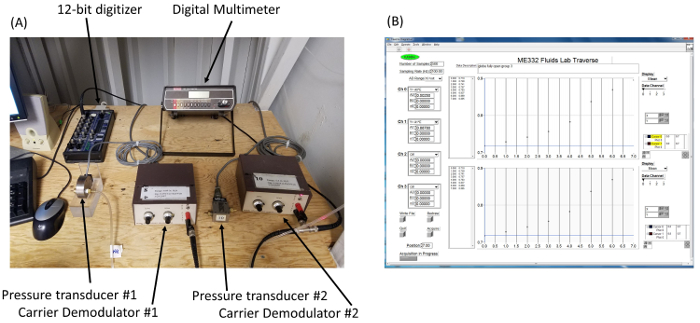
 ).
).
 . Consider the total loss coefficient as
  .
.Skip to...
Videos from this collection:

Now Playing
Conservation of Energy Approach to System Analysis
Mechanical Engineering
7.4K Views

Buoyancy and Drag on Immersed Bodies
Mechanical Engineering
30.0K Views

Stability of Floating Vessels
Mechanical Engineering
22.6K Views

Propulsion and Thrust
Mechanical Engineering
21.7K Views

Piping Networks and Pressure Losses
Mechanical Engineering
58.2K Views

Quenching and Boiling
Mechanical Engineering
7.7K Views

Hydraulic Jumps
Mechanical Engineering
41.0K Views

Heat Exchanger Analysis
Mechanical Engineering
28.0K Views

Introduction to Refrigeration
Mechanical Engineering
24.7K Views

Hot Wire Anemometry
Mechanical Engineering
15.6K Views

Measuring Turbulent Flows
Mechanical Engineering
13.5K Views

Visualization of Flow Past a Bluff Body
Mechanical Engineering
11.9K Views

Jet Impinging on an Inclined Plate
Mechanical Engineering
10.8K Views

Mass Conservation and Flow Rate Measurements
Mechanical Engineering
22.7K Views

Determination of Impingement Forces on a Flat Plate with the Control Volume Method
Mechanical Engineering
26.0K Views
Copyright © 2025 MyJoVE Corporation. All rights reserved