Long-term Video Tracking of Cohoused Aquatic Animals: A Case Study of the Daily Locomotor Activity of the Norway Lobster (Nephrops norvegicus)

Podsumowanie

Here we present a protocol to individually track animals over a long period of time. It uses computer vision methods to identify a set of manually constructed tags by using a group of lobsters as case study, simultaneously providing information on how to house, manipulate, and mark the lobsters.

Streszczenie

We present a protocol related to a video-tracking technique based on the background subtraction and image thresholding that makes it possible to individually track cohoused animals. We tested the tracking routine with four cohoused Norway lobsters (Nephrops norvegicus) under light-darkness conditions for 5 days. The lobsters had been individually tagged. The experimental setup and the tracking techniques used are entirely based on the open source software. The comparison of the tracking output with a manual detection indicates that the lobsters were correctly detected 69% of the times. Among the correctly detected lobsters, their individual tags were correctly identified 89.5% of the times. Considering the frame rate used in the protocol and the movement rate of lobsters, the performance of the video tracking has a good quality, and the representative results support the validity of the protocol in producing valuable data for research needs (individual space occupancy or locomotor activity patterns). The protocol presented here can be easily customized and is, hence, transferable to other species where the individual tracking of specimens in a group can be valuable for answering research questions.

Wprowadzenie

In the last few years, automated image-based tracking has provided highly accurate datasets which can be used to explore basic questions in ecology and behavior disciplines¹. These datasets can be used for the quantitative analysis of animal behavior^2,3. However, each image methodology used for tracking animals and behavior evaluation has its strengths and limitations. In image-based tracking protocols that use spatial information from previous frames in a movie to track animals^4,5,6, errors can be introduced when the paths of two animals cross. These errors are generally irreversible and propagate through time. Despite computational advances that reduce or almost eliminate this problem^5,7, these techniques still need homogeneous experimental environments for accurate animal identification and tracking.

The employment of marks that can be uniquely identified in animals avoids these errors and allows the long-term tracking of identified individuals. Widely used markers (e.g., barcodes and QR codes) exist in industry and commerce and can be identified using well-known computer vision techniques, such as augmented reality (e.g., ARTag⁸) and camera calibration (e.g., CALTag⁹). Tagged animals have previously been used for high-throughput behavioral studies in different animal species, for example, ants³ or bees¹⁰, but some of these previous systems are not optimized for recognizing isolated tags³.

The tracking protocol presented in this paper is especially suitable for tracking animals in one-channel imagery, such as infrared (IR) light or monochromatic light (particularly, we use blue light). Therefore, the method developed does not use color cues, being also applicable to other settings where there are constraints in the illumination. In addition, we use customized tags designed so as not to disturb the lobsters and, at the same time, allow recording with low-cost cameras. Moreover, the method used here is based on frame-independent tag detection (i.e., the algorithm recognizes the presence of each tag in the image regardless of the previous trajectories). This feature is relevant in applications where animals can be temporarily occluded, or animals' trajectories may intersect.

The tag design allows its use in different groups of animals. Once the parameters of the method are set, it could be transferred to tackle other animal-tracking problems without the need for training a specific classifier (other crustaceans or gastropods). The main limitations of exporting the protocol are the size of the tag and the need for attachment to the animal (which makes it not suitable for small insects, such as flies, bees, etc.) and the 2D assumption for the animal movement. This constraint is significant, given that the proposed method assumes the tag size remains constant. An animal moving freely in a 3D environment (e.g., fish) would show different tag sizes depending on its distance to the camera.

The purpose of this protocol is to provide a user-friendly methodology for tracking multiple tagged animals over a long period of time (i.e., days or weeks) in a 2D context. The methodological approach is based on the use of open source software and hardware. Free and open source software permits adaptations, modifications, and free redistribution; therefore, the generated software improves at each step^11,12.

The protocol presented here focuses on a laboratory set up to track and evaluate the locomotor activity of four aquatic animals in a tank for 5 days. The video files are recorded from a 1 s time-lapse image and compiled in a video at 20 frames per second (1 recorded day occupies approximately 1 h of video). All video recordings are automatically postprocessed to obtain animal positions, applying computer vision methods and algorithms. The protocol allows obtaining large amounts of tracking data, avoiding their manual annotation, which has been shown to be time-intensive and laborious in previous experimental papers¹³.

We use the Norway lobster (Nephrops norvegicus) for the case study; thus, we provide species-specific laboratory conditions to maintain them. Lobsters perform well-studied burrow emergence rhythms that are under the control of the circadian clock^14,15, and when cohoused, they form dominance hierarchy^16,17. Hence, the model presented here is a good example for researchers interested in the social modulation of behavior with a specific focus on circadian rhythms.

The methodology presented here is easily reproduced and can be applied to other species if there is a possibility to distinguish between animals with individual tags. The minimum requirements for reproducing such an approach in the laboratory are (i) isothermal rooms for the experimental setup; (ii) a continuous water supply; (iii) water temperature control mechanisms; (iv) a light control system; (v) a USB camera and a standard computer.

In this protocol, we use Python¹⁸ and OpenCV¹⁹ (Open Source Computer Vision Library). We rely on fast and commonly applied operations (both in terms of implementation and execution), such as background subtraction²⁰ and image thresholding^21,22.

Access restricted. Please log in or start a trial to view this content.

Protokół

The species used in this study is not an endangered or protected species. Sampling and laboratory experiments followed the Spanish legislation and internal institutional (ICM-CSIC) regulations regarding animal welfare. Animal sampling was conducted with the permission of the local authority (Regional Government of Catalonia).

1. Animal Maintenance and Sampling

NOTE: The following protocol is based on the assumption that researchers can sample N. norvegicus in the field during the night to avoid damage to the photoreceptors²³. Exposure of N. norvegicus to sunlight must be avoided. After sampling, the lobsters are supposed to be housed in an acclimation facility similar to the one reported on previously^17,24, with a continuous flow of refrigerated seawater (13 °C). The animals used in this study are male at the intermoult state with a cephalothorax length (CL; mean ± SD) of 43.92 ± 2.08 mm (N = 4).

1. Keep the individuals in isolated compartments to avoid any damages due to individual fights (see Figure 1a-d).
2. Feed them about 3x a week at random times to not interfere with the circadian rhythms.
   NOTE: In this experiment, mussels (approximately 4 g per lobster) were used as food. Mussels were bought from frozen food suppliers and were suitable for human consumption.
3. Use blue light (425 - 515 nm) to simulate light hours according to the spectral sensitivity of the species²⁵ and the environmental conditions at 400 m deep²⁶ (see Figure 1c,d).
   NOTE: The facility used here has a vertical ceiling of two blue (478 nm) fluorescent lamps that produced a light intensity of 12 lx at 1 m of distance from the lamps. See Figure 1a for the ceiling lamps' position and see the Table of Materials for the manufacturer's and technical lamps' characteristics.
4. Adjust the photoperiod of the acclimation facility to 12/12 light/darkness hours or simulate the natural photoperiod of the local latitude.
5. Regulate the facility temperature to 13 °C and monitor 2x daily to check the temperature of the inflowing seawater is around 13 °C (see Figure 1e).
6. Regulate the inflow of seawater at a rate of about 4 L/min to maintain good oxygenation.
   ​NOTE: The seawater circulates in an open circuit (no filters and additional pumps are used). The water supply depends on the main aquarium plant services.

Figure 1: Facility acclimation views. (a) Tank shelves. (a1) Seawater input. (a2) Fluorescent ceiling lights. (b) Detail of blue light illumination. (c) Animal cell detail. (d) Detail of an isolated facility control panel. (e) Temperature setting for one of the entrances. Please click here to view a larger version of this figure.

2. Tag's Construction

NOTE: The tag used here can be changed according to the characteristics of the target animal or other specific considerations.

1. Cut four circles of 40 mm in diameter from a black plastic sheet.
2. Cut from a white PVC plastic sheet two equilateral triangles with 26 mm sides.
3. Cut from a white PVC plastic sheet two circles of 26 mm in diameter.
4. Mark the center of the white triangles and circles and make a 10 mm hole in it.
5. Glue the four white shapes to the center of the four black circles.

Figure 2: The four tags used for the individual tagging of the lobsters. Circle, circle-hole, triangle, triangle-hole. Please click here to view a larger version of this figure.

3. Experimental Setup

NOTE: The experimental arena is supposed to be in an experimental chamber independent from but in close proximity to the acclimation facility.

1. Set up an experimental chamber where the air temperature can be controlled and maintained at the same temperature as the seawater in the experimental arena.
2. Modify a fiberglass tank (1,500 x 700 x 300 mm) to be used as an experimental arena. Add four burrows using PVC flexible pipes at the bottom of the tank and stick sand on the surface where the lobsters are supposed to move (Figure 3b-e). For more details, see^17,27.
   1. Provide the experimental arena with submergible blue LEDs (472 nm, simulating light hours) and IR LEDs (850 nm, dark conditions) (see also Figure 3a)^17,24.
      NOTE: LED light is used due to its low heat impact and the availability of usable electronic control and free hardware. An isolated facility with an environmental and seawater temperature of 13 ± 0.5 °C was used.
   2. Always keep the IR LEDs switched on.
      NOTE: The IR is needed to video record in dark conditions and in light conditions. It is not necessary to switch it off.
   3. Connect the blue LEDs with an apparatus to manage the photoperiod. See the suggestions in the Table of Materials, and for more details, consult Sbragaglia et al.¹⁷ (also shown in Figure 3a).
      NOTE: Illumination in video- or image-automated analyses is a critical factor. Regular illumination without shadows all over the arena avoiding water surface reflections makes the posterior video or image analysis easier. In the context of this protocol, only 12/12 light/darkness conditions were used. Light and darkness were gradually achieved within 30 min, and a light-controller script is added as Supplementary File 1.
   4. Place the chilled seawater inlet at one corner of the tank and the corresponding outlet at the opposite corner.
   5. Regulate the seawater input at a flow rate of about 4 L/min.
   6. Surround the tank with a black curtain in order to provide a full isolation from other light (Figure 3a).
3. Place the tripod to which the web camera is fixed to the side of the experimental arena and position the video camera above (130 cm) and at the center of the experimental arena (75 cm x 32.5 cm (see Figure 3a).
4. Check whether the video camera is in the centered position (see step 3.3) to make sure it has not been moved involuntarily.
5. Connect the web camera to a computer that is placed outside the curtain (Figure 3a).
   1. Install the software to manage the time-lapse recording with the video camera.
      NOTE: Time-lapse recordings depend on the movement's speed of the species. Also, see the Table of Materials for the camera, fisheye lens, PC, and software characteristics and manufacturers used here.
   2. Adjust the parameters of the video recording according to the characteristics of the species.
      NOTE: Considering the mobility rate of N. norvegicus, a 1 s time-lapse recording was used here, and the video was saved every 24 h.
   3. Make sure to create a timestamp (including the date) in the time-lapse video (as this can help for the future manual scoring of the behavior).

Figure 3: Experimental setup. (a) Diagram of the assembly of the experimental tank and video acquisition. (b) General view of the experimental tank. (c) Bottom view of the experimental tank, indicating the artificial burrows. (d) Top view, showing the bottom of the experimental tank. (e) Detail of one of the burrow entrances. Please click here to view a larger version of this figure.

4. Experimental Trial and Animal Preparation

NOTE: All steps with animals must be done in the acclimation facility and under red light conditions according to the spectral sensitivity of the Norway lobster²⁵. When moving the animals between the acclimation and the experimental facility, avoid any exposure of the lobsters to light, using an opaque black bag to cover the icebox.

1. Prepare an icebox previously separated into four submerged compartments with water at about 7 °C.
2. Prepare the four tags previously constructed and fast glue, like cyanoacrylate.
3. Prepare a tray with crushed ice.
4. Select the four lobsters to be tagged in the acclimation facility and put each of them in a compartment of the icebox.
5. Wait 30 min and, then, start the tagging procedure.
   1. Take a lobster and put it on the crushed ice for 5 min to immobilize it and facilitate the tagging operation.
   2. Dry the upper part of the lobster's cephalothorax with adsorptive paper and put a drop of fast glue on it.
   3. Place the tag horizontally on top of the animal's cephalothorax, in contact with the glue, and wait enough time for it to harden (for about 20 s).
   4. Return the lobster to its compartment in the icebox and proceed with the other three animals in the same way.
   5. Put the lobsters back in the cell where they were previously and wait for 24 h to be sure that the tag is properly glued on.
   6. Transfer the lobsters from the acclimation facility to the experimental chamber using the same icebox that was used for the tagging procedure.
6. Launch the video recording and wait 5 min before introducing the tagged lobsters. Obtain an averaged background image from the initial 100 frames.
   NOTE: Waiting a minimum of 1 min is mandatory to obtain background frames without tagged lobsters; they are needed for video processing.
7. Introduce the animals one by one in the experimentation tank inside their respective compartment, keeping the water in it.
8. Wait for them to get out; if they do not come out, help them gently by tilting the compartment. See Figure 4 as example of the animals inside the tank under experimental conditions.

Figure 4: Raw video frame. An example of a representative frame from one of the time-lapse videos collected during the experiments. At the upper right corner, we show the time stamp with the date, time, and frame. Notice the differences in the tank illumination in the image's lower corner. Please click here to view a larger version of this figure.

5. Video Analysis Script

1. Perform the analysis after completion of the experiment.
   1. Launch the computer vision script for video analysis.
   2. Launch Java program to calculate the positions and distance covered by the lobsters and insert the data in the database.
      NOTE: This program is a Euclidean distance-based algorithm²⁸.
   3. Launch SQL script to binning data as desired time interval (ex. 10 min).

6. Computer Vision Script for Video Analysis

NOTE: The script avoids fisheye image correction because it does not introduce a relevant error in the experimental setup. Nonetheless, it is possible to correct this with OpenCV camera calibration functions²⁹ based on vector and matrix rotation methods^30,31.

1. Select the Python¹⁸ program language.
2. Select the OpenCV¹⁹ image and video processing library.
3. Load a video.
   NOTE: Video formats .avi or .mp4 were used in this experiment, but this is not mandatory. It depends on the FourCC³² codecs installed in the operating system.
4. Perform the following steps for each frame Fi in the video.
   1. Subtract the background²⁰ B (average of the last 100 frames, obtained from step 4.6) from the current frame Fi, and update the background image B as Fi. Use the function BackgroundSubtractorMOG2 from the OpenCV¹⁹ library (see the scripts in the Supplementary File 2).
   2. Determine the set of regions of interest (ROIs) R from the pixels with relevant motion indicated by the background subtractor. Use the method apply from BackgroundSubtractorMOG2 in the OpenCV¹⁹ library (see the scripts in the Supplementary File 2). In the set, include the animal detections from the previous frame, to take into account nonmoving animals.
   3. Perform the following steps for each ROI Ri
      1. Apply the dilate function and compute the contours³³ of ROI Ri. Use the functions dilate and findContours from the OpenCV¹⁹ library (see the scripts in the Supplementary File 2).
      2. Compute the hull area³⁴ hi in the number of pixels. Use the function convexHull from the OpenCV¹⁹ library (see the scripts in the Supplementary File 2).
      3. Compute the radius³⁵ ri of the ROI Ri. Use the function minEnclosingCircle from the OpenCV¹⁹ library (see the scripts in the Supplementary File 2).
      4. Compute the solidity si of the ROI Ri. Solidity is the ratio of the contour area (obtained in step 6.4.3.1) to its convex hull area (obtained in step 6.4.3.2) of the Ri.
      5. Compute the aspect ratio ai of the ROI Ri. Aspect ratio is the ratio between the width and the height of the Ri-bounding rectangle. The bounding rectangle is computed using the function boundingRect from the OpenCV¹⁹ library.
   4. Select a reduced set of ROIs as a candidate to contain the animals, by adjusting the properties for hull area, radius, solidity, and aspect ratio.
      1. Check if hi is less than 500.0 or greater than 100000.0. If so, discard the ROI Ri. Otherwise, keep the Ri as a candidate ROI for the animal location.
      2. Check if the ri is less than 40.0. If so, discard the ROI Ri. Otherwise, keep the Ri as a candidate ROI for the animal location.
      3. Check if the si is less than -4.0 discard the ROI Ri. Otherwise, keep the Ri as a candidate ROI for the animal location.
      4. Check if the ai is less than 0.15 or greater than 4.0. Is so, discard the ROI Ri. Otherwise, keep the Ri as a candidate ROI for the animal location.
         NOTE: The use of ROIs reduces the computational cost, focusing the tag search on the animal's body region. Animal detections from previous frames are included to avoid wrong detections when the animals are not moving.
   5. Analyze the animal ROIs to determine the tag identities. Execute de following steps for each ROI Ri and for each internal ROI Pi, and extract the internal ROIs P.
      1. Binarize the grayscale image Pi using the Otsu³⁶ thresholding algorithm.
      2. Compute the contours³³ of Pi, as in step 6.4.3.1.
      3. Compute the hull area³⁴ hi and the aspect ratio ai, as in steps 6.4.3.2 and 6.4.3.5.
      4. Compute the shape moments^37,38 mi of Pi. Use the function moments from the OpenCV¹⁹ library (see the scripts in the Supplementary File 2).
      5. Select a reduced set of ROIs as a candidate to contain the tags, using the following criteria.
         1. Check if hi is less than 150.0 or greater than 500.0. If so, discard the ROI Pi. Otherwise, keep the Pi as a candidate ROI for the tag location.
         2. Check if the ai is less than 0.5 or greater than 1.5. If so, discard the ROI Pi. Otherwise, keep the Pi as a candidate ROI for the animal location.
         3. Check if the mi is greater than 0.3. If so, discard the ROI Pi. Otherwise, keep the Pi as a candidate ROI for the animal location.
   6. Classify the tag ROIs. Approximate a polygon³⁹ using the OpenCV¹⁹ function³⁸ for each selected ROI Pi¹⁹.
      1. Check if there are exactly three vertices in the approximated polygon; assign the tag to the triangle class. Otherwise, assign the circle class to the tag region.
         NOTE: Approximated polygon is stored using a matrix with the vertices.
      2. Check the central pixel of the ROI Pi. If it is a black pixel, assign the Pi to the holed class. Otherwise, assign the Pi to the white class.
         NOTE: The shape center is deduced from the moments calculated in step 6.4.5.4. Search the black pixels in an area of a 4-pixel radius around the center.
5. Save the frame data: frame date, frame time, shape class, x center shape coordinate, and y center shape coordinate.
6. Continue with the next frame or end the process. See Figure 5 below as a visual example of the working script steps and watch Video 1 as an example of script functioning.

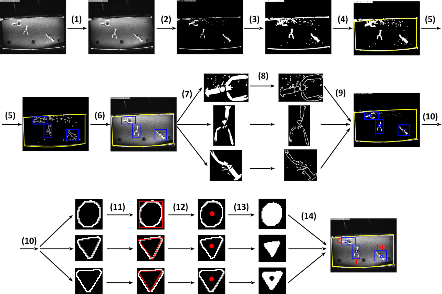
Figure 5: Relevant steps of the video-processing script. (1) Evaluate the background subtraction motion over the mean of the last 100 frames. (2) Result of the background subtraction algorithm. (3) Apply a dilate morphological operation to the white-detected areas. (4) Apply fix, static, main ROI; the yellow polygon corresponds to the bottom tank area. (5) Calculate contours for each white-detected region in the main ROI and perform a structural analysis for each detected contour. (6) Check structural property values and, then, select second-level ROI candidates. (7) Binarize the frame using an Otsu thresholding algorithm; the script works only with second-level ROIs. (8) For each binarized second-level ROI, calculate the contours of the white regions and perform a structural analysis for each detected contour. (9) Check the structural property values and, then selects internal ROI candidates. (10) For each contour in the internal ROI candidate, calculate the descriptors/moments. (11) Check if the detected shape matches with the model shape and approximate a polygon to the best match candidates. (12) Check the number of vertices of the approximate polygon and determine the geometric figure: circle or triangle. (13) Calculate the figure center and check if black pixels occur; if yes, it is a holed figure. (14) Visual result after frame analysis. Please click here to view a larger version of this figure.

Access restricted. Please log in or start a trial to view this content.

Wyniki

We manually constructed a subset of the experimental data to validate the automated video analysis. A sample size of 1,308 frames with a confidence level of 99% (which is a measure of security that shows whether the sample accurately reflects the population, within its margin of error) and a margin of error of 4% (which is a percentage that describes how close the response the sample gave is to the real value in the population) was randomly selected, and a manual annotation of the correct...

Access restricted. Please log in or start a trial to view this content.

Dyskusje

The performance and representative results obtained with the video-tracking protocol confirmed its validity for applied research in the field of animal behavior, with a specific focus on social modulation and circadian rhythms of cohoused animals. The efficiency of animal detection (69%) and the accuracy of tag discrimination (89.5%) coupled with the behavioral characteristics (i.e., movement rate) of the target species used here suggest that this protocol is a perfect solution for long-term experimental trials (e.g., da...

Access restricted. Please log in or start a trial to view this content.

Materiały

Name	Company	Catalog Number	Comments
Tripod 475	Manfrotto	A0673528	Discontinued
Articulated Arm 143	Manfrotto	D0057824	Discontinued
Camera USB 2.0 uEye LE	iDS	UI-1545LE-M	https://en.ids-imaging.com/store/products/cameras/usb-2-0-cameras/ueye-le.html
Fish Eye Len C-mount f = 6 mm/F1.4	Infaimon	Standard Optical	https://www.infaimon.com/es/estandar-6mm
Glass Fiber Tank 1500 x 700 x 300 mm3
Black Felt Fabric
Wood Structure Tank			5 Wood Strips 50x50x250 mm
Wood Structure Felt Fabric			10 Wood Strips 25x25x250 mm
Stainless Steel Screws			As many as necessary for fix wood strips structures
PC			2-cores CPU, 4GB RAM, 1 GB Graphics, 500 GB HD
External Storage HDD			2 TB capacity desirable
iSPY Sotfware for Windows PC	iSPY		https://www.ispyconnect.com/download.aspx
Zoneminder Software Linux PC	Zoneminder		https://zoneminder.com/
OpenCV 2.4.13.6 Library	OpenCV		https://opencv.org/
Python 2.4	Python		https://www.python.org/
Camping Icebox
Plastic Tray
Cyanocrylate Gel			To glue tag’s
1 black PVC plastic sheet (1 mm thickness)			Tag's construction
1 white PVC plastic sheet (1 mm thickness)			Tag's construction
4 Tag’s Ø 40 mm			Maked with black & white PVC plastic sheet
3 m Blue Strid Led Ligts (480 nm)			Waterproof as desirable
3 m IR Strid Led Ligts (850 nm)			Waterproof as desirable
6 m  Methacrylate Pipes Ø 15 mm			Enclosed Strid Led
4 PVC Elbow  45o Ø 63 mm			Burrow construction
3 m Flexible PVC Pipe Ø 63 mm			Burrow construction
4 PVC Screwcap Ø 63 mm			Burrow construction
4 O-ring Ø 63 mm			Burrow construction
4 Female PVC socket glue / thread Ø 63 mm			Burrow construction
10 m DC 12V Electric Cable			Light Control Mechanism
Ligt Power Supply DC 12 V 300 W			Light Control Mechanism
MOSFET, RFD14N05L, N-Canal, 14 A, 50 V, 3-Pin, IPAK (TO-251)	RS Components	325-7580	Light Control Mechanism
Diode, 1N4004-E3/54, 1A, 400V, DO-204AL, 2-Pines	RS Components	628-9029	Light Control Mechanism
Fuse Holder	RS Components	336-7851	Light Control Mechanism
2 Way Power Terminal 3.81 mm	RS Components	220-4658	Light Control Mechanism
Capacitor 220 µF 200 V	RS Components	440-6761	Light Control Mechanism
Resistance 2K2 7 W	RS Components	485-3038	Light Control Mechanism
Fuse 6.3 x 32 mm2 3A	RS Components	413-210	Light Control Mechanism
Arduino Uno Atmel Atmega 328 MCU board	RS Components	715-4081	Light Control Mechanism
Prototipe Board CEM3,3 orific.,RE310S2	RS Components	728-8737	Light Control Mechanism
DC/DC converter,12 Vin,+/-5 Vout 100 mA 1 W	RS Components	689-5179	Light Control Mechanism
2 SERA T8 blue moonlight fluorescent bulb 36 watts	SERA		Discontinued/Light isolated facility