Method Article
PyDesigner v1.0: A Pythonic Implementation of the DESIGNER Pipeline for Diffusion Magnetic Resonance Imaging
* These authors contributed equally
In This Article
Summary
Here we present PyDesigner, a Python-based diffusion magnetic resonance imaging (dMRI) processing pipeline capable of correcting for typical dMRI artifacts and producing diffusion tensor imaging (DTI), diffusion kurtosis imaging (DKI), fiber ball imaging (FBI), microstructure modeling (white matter integrity [WMTI] and fiber ball white matter [FBWM]), and tractography outputs.
Abstract
PyDesigner is a Python-based software package based on the original Diffusion parameter EStImation with Gibbs and NoisE Removal (DESIGNER) pipeline (Dv1) for dMRI preprocessing and tensor estimation. This software is openly provided for non-commercial research and may not be used for clinical care. PyDesigner combines tools from FSL and MRtrix3 to perform denoising, Gibbs ringing correction, eddy current motion correction, brain masking, image smoothing, and Rician bias correction to optimize the estimation of multiple diffusion measures. It can be used across platforms on Windows, Mac, and Linux to accurately derive commonly used metrics from DKI, DTI, WMTI, FBI, and FBWM datasets as well as tractography ODFs and .fib files. It is also file-format agnostic, accepting inputs in the form of .nii, .nii.gz, .mif, and dicom format. User-friendly and easy to install, this software also outputs quality control metrics illustrating signal-to-noise ratio graphs, outlier voxels, and head motion to evaluate data integrity. Additionally, this dMRI processing pipeline supports multiple echo-time dataset processing and features pipeline customization, allowing the user to specify which processes are employed and which outputs are produced to meet a variety of user needs.
Introduction
Diffusion MRI (dMRI) is widely applied for the noninvasive study of microstructural properties in the brain. While many dMRI methods have been proposed, two commonly used are diffusion tensor imaging (DTI) and diffusional kurtosis imaging (DKI). These techniques are closely related, with DKI being an extension of DTI that includes quantification of diffusional non-Gaussianity1. Both provide a variety of scalar diffusion measures and enable the construction of white matter fiber tractography. An important advantage of DTI and DKI is that they have a solid foundation in diffusion physics so that their validity does not rely on detailed assumptions regarding tissue microstructure2,3. This allows DTI and DKI to be applied throughout the brain and body for participants of any age and disease status.
Because raw diffusion-weighted images (DWIs) are degraded by multiple factors, including signal noise, motion, Gibbs ringing, and eddy current distortion, preprocessing should be employed prior to the calculation of any diffusion quantities4. Preprocessing of DWIs is an active field of research that is now highly developed. However, combining the necessary processing steps into a single pipeline that gives consistent results is challenging because several user-defined settings must be adjusted depending on the details of the dMRI acquisition and because the order in which the preprocessing steps are performed affects the outcome. For this reason, the Diffusion parameter EStImation with Gibbs and NoisE Removal (DESIGNER, GitHub: NYU-DiffusionMRI/DESIGNER) pipeline was initially proposed in 2016 to optimize, standardize, and streamline the preprocessing for DWIs5. DESIGNER Dv1 relies on software tools that are embedded in FSL, MRtrix3, MATLAB, and Python to create a seamless and complete DWI process - one that encompasses image correction through preprocessing and diffusion/kurtosis tensor estimation5. With control flags to toggle preprocessing steps on or off, DWI corrections can be performed selectively. DESIGNER preprocesses in a specific order - (i) Marchenko-Pastur principal component analysis (MP-PCA) denoising6, (ii) Gibbs ringing correction7, (iii) echo-planar imaging (EPI) distortion correction8, eddy current correction9, motion correction10, and outlier replacement11, (iv) B1 bias field correction, (v) brain mask generation, (vi) smoothing, (vii) Rician noise bias correction, and (viii) b0 normalization. Preprocessing in this specific order improves both accuracy and the effective signal-to-noise ratio (SNR)5. It is worth noting that each step of PyDesigner is optional and can be employed or skipped based on user preference. Smoothing, for example, may not be a necessary preprocessing step for some datasets. Though it helps to mitigate filtering errors, it may not be needed for ultra-high-quality datasets. As such, users can choose to employ only the steps needed for their data.
Implementing DESIGNER across platforms is challenging due to differences in operating systems and environment settings. In particular, the fact that DESIGNER Dv1 is primarily written in MATLAB creates significant portability issues arising from complicated configuration requirements needed to enable Python-MATLAB interfacing. Moreover, different combinations of MATLAB, Python, and dependency versions compromise the reproducibility of this pipeline. For this reason, we have developed PyDesigner, which is entirely Python-based. Not only does this dMRI processing pipeline allow for seamless preprocessing, but it also allows the pipeline to be incorporated into a Docker container, which greatly enhances portability and reproducibility. Additionally, by replacing the MATLAB code, PyDesigner avoids all licensing fees and improves accessibility.
This dMRI processing pipeline augments the hands-free approach introduced by DESIGNER, adds several new features, and incorporates tools from FSL and MRtrix3 to perform preprocessing. Standard mathematical Python libraries such as Numpy12, SciPy13, and CVXPY14,15 were used to replace the MATLAB portions of DESIGNER with Python code. This software is openly provided and available on Github16. The goal of this paper is not to validate or compare our software to similar software but rather to give users a step-by-step guide for processing their data with PyDesigner should they choose to do so.
Protocol
All data used to develop and test the software was collected under an institutional review board-approved study protocol.
NOTE: PyDesigner was built on MacOS 10.14 and requires a Windows Subsystem for Linux (WSL) to run on Windows. The same commands can be used for Linux/Mac systems.
1. Operating system compatibility
- For Windows systems follow the link to install WSL17 and then proceed to step 2.6.
- For Unix-based systems (such as Linux and Mac) proceed to section 2.
NOTE: Unix-based systems can natively install PyDesigner and its dependencies.
2. Install FSL
NOTE: All PyDesigner testing has been done with FSL version 6.0.2, and using v6.0.2 or above is recommended.
- Go to the FSL wiki18 and select Download/Install. For Windows users, go to step 2.6.
- Choose Download FSL under the Installing FSL heading. Then select the FSL Install Software License, read the agreement, and select agree.
- Fill out the required fields and select Register.
- Choose the Download FSL link (first link on the page). Then select the installation instructions link (second link on the page). Follow these instructions to download FSL for each operating system.
NOTE: FSL takes about 10 min to install. - To verify successful installation, enter the following into a new terminal window:
$ flirt -version. This should return the version number. Proceed to step 3. - For Windows users, follow the WSL installation guide for FSL19.
3. Create a Conda environment
- Install a conda package to manage Python environments. Users can choose either Miniconda or Anaconda.
- Download Miniconda/Anaconda20. Mac and Linux users proceed to step 3.2.
- For Windows, set up conda within WSL21.
NOTE: The following instructions are for Miniconda, but the same commands work for Anaconda. Although conda no longer supports Python 3.7, it is still possible to create a conda environment with Python 3.7, allowing this protocol to be implemented precisely as described.
- Enter the following into the terminal to create the conda environment:
$ conda create -n mri python=3.7. Use this conda environment for all PyDesigner-related activities.- When prompted with
Proceed ([y]/n)?Entery.
NOTE: -n flag: Use this to indicate the name of the conda environment. In the video, the conda environment is named mri.
NOTE:python=: Version 3.7 is recommended, as PyDesigner was built and tested on this version.
- When prompted with
4. Install MRtrix3
- Activate the conda environment by entering the following command:
$ conda activate mri - Open the download page for MRtrix322 and follow the download instructions for the appropriate operating system. The installation code will ask for confirmation of certain dependencies. Enter
yto continue the download process.- Print the MRtrix3 documentation to confirm installation by entering the following into the terminal:
$ mrinfo -h
- Print the MRtrix3 documentation to confirm installation by entering the following into the terminal:
5. Install PyDesigner
- Open a new terminal window and activate the conda environment by entering the following into the terminal:
$ conda activate mri - Run the command:
$ pip install PyDesigner-DWI - To verify successful installation, print the version number by entering the following into the terminal:
$ pydesigner -v- If the error "module not found" appears, please see the Troubleshooting section at the end of the protocol (section 10)
NOTE: $ pydesigner -h will print help documentation that explains the commands and syntax for the software. PyDesigner can also be downloaded via Github. See the installation instructions on the website23.
- If the error "module not found" appears, please see the Troubleshooting section at the end of the protocol (section 10)
6. Data preparation
NOTE: PyDesigner works with multiple file types such as .nii, .nii.gz, .mif and DICOM. In the video, DICOMs are sorted and converted to NIfTI before using this dMRI processing pipeline. NIfTI files are easier to work with because they are deidentified, and there is one file per sequence.
- To sort the DICOMs, use the DicomSort tool24.
NOTE: Any other DICOM sorting tool available that accomplishes the same task is allowable. - After sorting the DICOMs, convert them to NIfTI files using dcm2niix25.
- Install dcm2niix by entering the following command into the terminal:
$ sudo apt installdcm2niix - Once downloaded, type the following into the terminal to verify the installation by printing the documentation for dcm2nii:
$ dcm2niix -h
- Install dcm2niix by entering the following command into the terminal:
- To run dcm2niix, enter the following command into the terminal:
$ dcm2niix -f %s_%p_%d -o pathtosavefolder/ pathtorawdicoms/
NOTE: -f: To specify the filename structure for the output file, follow this tag with any desired filename structure. The video uses: -f %s_%p_%d . %s, %p and %d are notations for series, protocol number, and description, respectively. Any file structure will work. Expected outputs from dcm2niix are .bval, .bvec, .json, and .nii files. If TOPUP data was acquired there will be .json and .nii TOPUP files.
7. Basic PyDesigner usage
NOTE: PyDesigner can take up to 1.5 h for a single data set depending on processing parameters and computer capabilities.
- To run standard processing, use the flag
-sor-standard. This command will run the recommended preprocessing pipeline in the following order: Denoising6, Gibbs-ringing correction7, EPI distortion correction8, eddy current motion correction9, creation of brain and cerebrospinal fluid (CSF) masks, smoothing, Rician bias correction, outlier detection11, tensor estimate, and creation of parametric maps. - To run the basic PyDesigner command, first activate the conda environment by entering the following command into the terminal:
$ conda activate mri - Print the help documentation for the software by entering the following command:
$ pydesigner -h. This documentation explains all possible commands and syntax for PyDesigner. - Use the following example to structure the command.
$ pydesigner -s --verbose --rpe_pairs 1 -o ./output_folder/ ./input_folder/input1.nii ./input_folder/input2.nii - Note the following important flags:
--verbose: Use this to view the PyDesigner console as it processes data (not required).--rpe pairs #: Use this to allow users with a TOPUP sequence to speed up the EPI distortion correction8 process by using TOPUP. The # refers to how many B0 volumes from the TOPUP sequence will be used. Using #=1 prevents overestimation of the distortion field and cuts down on the time needed to create this field. Users have routinely used #=1 with reliable results. When using #=1 PyDesigner will default to taking the first volume.
8. Advanced PyDesigner usage: Tailoring the software to the users' individual needs
NOTE: When tailoring PyDesigner, omit the -s flag; this flag is the command for automatic preprocessing.
- Activate the conda environment by entering the following command into the terminal:
$ conda activate mri - Consult the software's website23 for a list of flags; each flag allows the user to run each part of PyDesigner individually.
- Structure the command. Start with the flags for each sequence that the user would like to perform. Then, direct PyDesigner to the input and output files. For example:
$ pydesigner flag1 flag2 flag3 -o ./output_folder/ ./input_folder/input1.nii - Example 1: Run tensor fitting alone (no additional preprocessing).
- Activate the conda environment by entering the following command into the terminal:
$ conda activate mri - Consult the PyDesigner website23 for a list of flags. This example uses
-m. -m: Add this flag to limit tensor fitting to within brain voxels only. This speeds up tensor fitting + outlier detection.- Use the following example to structure the command:
$ pydesigner -m -o ./output_folder/ ./input_folder/input1.nii
NOTE: The input for tensor fitting is a preprocessed .nii file.
- Activate the conda environment by entering the following command into the terminal:
- Example 2 Run denoising alone (no additional preprocessing).
- Activate the conda environment by entering the following into the terminal:
$ conda activate mri - Consult the PyDesigner website23 for a list of flags. This example uses
-n. - -n: Add this flag to complete the denoising step. Input the previously preprocessed DWI file labeled DWI_preproccessed.nii, which is found in each subject's output folder.
- Use the following example to structure the command:
$ pydesigner -n -o ./output_folder/ ./input_folder/input1.nii
- Activate the conda environment by entering the following into the terminal:
9. Future PyDesigner updates
NOTE: Updates can be found on the website23.
- To update PyDesigner, enter the following into a new terminal window:
$ pip install --upgrade PyDesigner-DWI
NOTE: If PyDesigner was installed through Github16, it must also be updated using git.
10. Troubleshooting Installation
- When downloading PyDesigner, the error code "module not found" will appear if there is a missing Python module.
- Fix a missing module by entering the following into the terminal:
$ pip install nameofmodule - Then repeat the first install command by entering the following into the terminal :
$ pip install PyDesigner-DWI - PyDesigner should now be fully installed. Please return to step 5.3. If the same error occurs, repeat this process until all missing Python modules are installed.
- Fix a missing module by entering the following into the terminal:
11. Troubleshooting output errors
- If any issues occur, review the log_command.json file to identify any preprocessing errors. Review the intermediate files to determine the specific error.
- For help troubleshooting, submit a request on the GitHub page16.
12. Running PyDesigner with an example dataset
- Download the example dataset from OpenNeuro here26.
NOTE: This example dataset contains both raw and preprocessed data. The raw data is intended as the input for PyDesigner example processing. The preprocessed data consists of the outputs generated after the raw data were processed using the dMRI processing pipeline on an iMac OS v12.4. Users can download the raw data, process these data using PyDesigner, and compare their outputs to the example outputs provided to ensure that PyDesigner is running correctly. Raw data is contained in the main folder (/PyDesigner Example Dataset/sub-01) and the preprocessed data is contained in the derivatives folder (/PyDesigner Example Dataset/derivatives/sub-01). Unless otherwise specified, the OpenNeuro dataset will download into the default user folder. - Open a new terminal on Mac/Linux or the WSL on Windows.
NOTE: To run the standard PyDesigner processing pipeline, follow the example command structure below. Enter the following commands below into the terminal/WSL. In this example, where " ./user_download_folder/" indicates the path for the example data folder. This path will be specific to where the example data is stored on the individual users computer. - To make a new folder for outputs, enter the following into the terminal:
$ mkdir ./user_download_folder/ ds004945-download /PyDesigner_Outputs - To activate the conda environment, enter the following into the terminal:
$ conda activate mri - To run PyDesigner on the example dataset, enter the following into the terminal:
$ pydesigner - o ./user_download_folder/ds004945-download/PyDesigner_Outputs -s ./user_download_folder/ds004945-download/sub-01/dwi/sub-01_dwi.nii
NOTE: In this example, ./user_download_folder/ indicates the path for the example data folder. This path will be specific to each user's computer. The commands in steps 12.3 to 12.5 follow the structure of step 8.3. This command employs the -s flag, PyDesigner's standard processing flag, which runs the following processing steps in this order: denoising6, Gibbs ringing correction7, undistortion8,9, brain masking, smoothing, and rician bias correction. - If the software is installed correctly, all outputs will populate in the newly created PyDesigner_Outputs folder. Compare the preprocessing files produced by PyDesigner with the example dataset preprocessed folder found in the "derivatives" folder downloaded from OpenNeuro.
- Consult the representative results section to compare their metric maps to those in the example dataset results.
Results
The PyDesigner software applies multiple image correction steps to raw diffusion data and generates outputs used to improve accuracy over the raw files when conducting analysis. Each step available in the pipeline has been previously validated through peer-reviewed publications5,6,7,8,9,10,11 as discussed in the introduction. The outputs from the software can be used in analyses such as tractography profiles, connectivity matrices, voxel-wise analyses, ROI analyses, fODF analyses, TBSS, and fixel-based analyses.
The software website23 lists all output files generated during the preprocessing pipeline. After each prompt is run, the console will output a description of all completed processes. There are 3 types of output files: processing files, metrics, and quality control. The output directory structure is shown in Figure 1. These files are available when using standard preprocessing (refer to section 7 of the protocol). If the user requires more advanced usage (refer to section 8 of the protocol), the output files available will be dependent on which processes were completed.
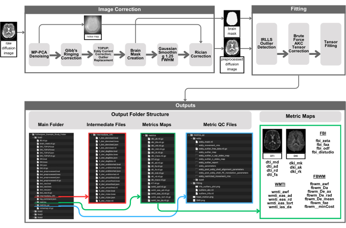
Figure 1: Visual representation of the PyDesigner pipeline. Preprocessing begins by providing an input 4D DWI to PyDesigner (top left), which then undergoes MP-PCA denoising to yield a denoised 4D DWI and a 3D noise map. The denoised 4D DWI then undergoes Gibbs ringing correction, Rician bias correction, TOPUP, eddy current correction, and outlier correction. A brain mask is then computed for subsequent steps, outlier detection, and tensor fitting to speed up computations by performing them within the brain mask only. Outputs can be found in subdirectories in the main subject processing folder - intermediate_nifti, metrics, and metrics_qc. Note that the screenshots of PyDesigner outputs are not meant to be an exhaustive list of all possible outputs but rather to provide a schematic visual example of what users can expect. Outputs, both final outputs and intermediate files, will vary based on user input data and processing flags employed. Please click here to view a larger version of this figure.
Processing
Processing files are used during the PyDesigner pipeline and are stored in the root output directory. For each preprocessing step, intermediate DWI files are saved in the output folder "intermediate_nifti" as shown in Figure 1. These files should be referenced when addressing any issues with processing or outputs to evaluate each step of the pipeline separately.
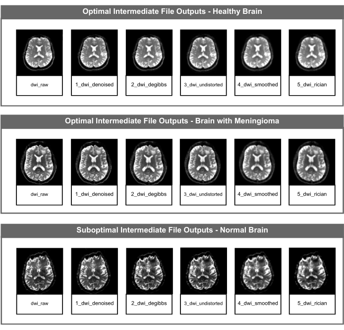
Figure 2: Optimal and suboptimal intermediate DWI NifTI files. The figure shows the intermediate NIfTI file for each image correction step of the PyDesigner pipeline. The top row is an example of optimal intermediate file outputs using data from a healthy adult brain, the middle row is an example of optimal intermediate file outputs using data from a pathological brain (meningioma), and the bottom row displays suboptimal intermediate file outputs using data from a healthy adult brain with a susceptibility artifact unrelated to brain structure or health. Please click here to view a larger version of this figure.
Metrics
This folder contains all the parametric maps that PyDesigner calculates (see Figure 1). This includes parametric maps for DTI/DKI, fiber ball imaging (FBI)/ fiber ball white matter (FBWM), and white matter tract integrity (WMTI) metrics (Table 1)16.

Table 1: Expected range of values for DTI/DKI and FBI/FBWM metrics. The table includes a list of robust DTI, DKI, FBI, and FBWM metrics generated by PyDesigner and their expected value ranges. The required sequences and b-values(s/mm2) to derive each metric are also listed. The DTI metrics listed are FA, MD, AD, and RD. The DKI metrics listed are MK, AK, RK, and KFA. The FBI metric listed is FAA. The FBWM metrics listed are AWF, DA, DE_AX, DE_RAD, and FAE.
Users can conduct visual and value quality control (QC) of the mean diffusivity (MD), fractional anisotropy (FA), and mean kurtosis (MK) metrics to identify suboptimal results. If these metrics are suboptimal by the standards described below, users should look at each intermediate file described in Figure 2 to determine which preprocessing step was unsuccessful.
Visual QC is used to identify suboptimal results (e.g., tensor fitting issues, and artifacts). We recommend using ImageJ for visual QC to ensure no manipulation is done to the image via software defaults. The top row of Figure 3 shows typical MD, FA, and MK metric maps using a biologically plausible threshold of 0-3 µm2/ms, 0-1 µm2/ms, and 0-2 µm2/ms, respectively (Figure 3 [Top row]). The MD map should have the highest values in the ventricles and high values in cortical grey matter (Figure 3A [Top row]). The FA map should have apparent white matter tracts that are clear throughout the brain (Figure 3B [Top row]). The MK map should have high values in WM and lower values in the grey matter and CSF (Figure 3C [Top row]). Figure 3D [Top row] is an example of a metric map with tensor fitting issues, which results in clusters of zero-value voxels. If any issues occur, review the log_command.json file to find any preprocessing errors. Review the intermediate files to determine the specific error. For help troubleshooting, submit a request on the PyDesigner GitHub page.
Value quality control is used to identify if the voxels of a given metric map are relatively uniform between subjects for each dataset. The expected value range for each map and dataset is dependent on the data and the PyDesigner parameters. In our test dataset, we had consistent peaks in the 8000 to 10,000, 2500 to 4000, and 5000 to 13,000 ranges for MD, FA, and MK, respectively, using FSLeyes default histogram binning. The bottom row of Figure 3 provides examples of histogram variability. Table 1 contains the expected x-axis values for these metrics. Higher or lower voxels are characteristic of the dataset or indicate an artifact or preprocessing issue (Figure 3D [Bottom row]).
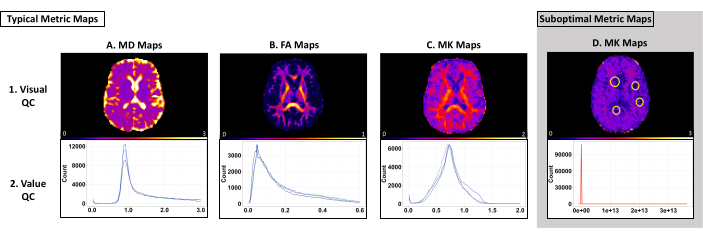
Figure 3: Example metric maps and histograms from PyDesigner with optimal and suboptimal results. The top row shows examples of single-subject MD, FA, and MK maps used for visual QC. The bottom row shows multi-subject histograms used for value QC. (A-C) Typical examples of metric maps and histograms that pass visual and value quality control. Each blue line on the histograms for each metric type represents an individual dataset. Note that each dataset follows a similar curve and falls within a similar range. (D) An example of a metric map that does not pass visual or value quality control. Note how the red line on the histogram shows a curve that differs from that of A-C. The zero voxels circled on this metric map are due to tensor fitting issues during preprocessing (Panel D, top row). This histogram is an example of generally higher or lower voxels in a dataset than expected (Panel D, bottom row). Please click here to view a larger version of this figure.
Quality control
Once PyDesigner has processed the data, the metrics_qc folder (see Figure 1) should be used to identify suboptimal datasets. For each dataset, PyDesigner outputs three plots used for quality control.
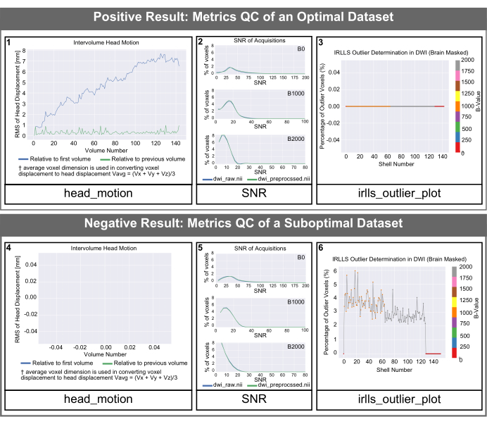
Figure 4: PyDesigner-generated QC histogramsfor optimal and suboptimal datasets. SNR, intervolume head motion, and outlier histograms generated by PyDesigner. Both rows represent data from a healthy adult brain. The top row is an example of quality control histograms for an optimal dataset. The bottom row shows quality control outputs of a suboptimal dataset with a susceptibility artifact unrelated to brain structure or health. Please note that the text size of the labels in the default outputs from PyDesigner is smaller than they will appear in this figure. We have increased the text size in this figure for readability. Please click here to view a larger version of this figure.
The head_motion graphs in Figure 4 show head displacement relative to the first volume and the previous volume. As seen in Figure 4 (panel 1), head displacement is typically small and PyDesigner adjusts for these motion artifacts in the standard processing pipeline using the FSL program Eddy along with TOPUP for motion and eddy current motion correction9. For suboptimal datasets, the head_motion graph may appear empty, as shown in Figure 4 (panel 4). This indicates that eddy current motion correction was unsuccessful therefore the PyDesigner was unable to output a graph. The Eddy current correction log files can be found in the eddy subfolder within the metrics_qc folder (see Figure 1). The signal-to-noise ratio (SNR) graph displays 3 plots. Each plot is for a different b-value and shows both the preprocessed and raw data. For an optimal dataset, the raw data SNR peak should be ≥5 (Figure 4 [panel 2]). Suboptimal datasets will have a raw data SNR peak of ≤3 (Figure 4 [panel 5]). Ideally, users should see that the SNR peak for all b-values increases slightly but not dramatically. The outlier plot is found in the fitting folder within metrics_qc and shows the percentage of outliers in the dataset (Figure 4 [panel 3 and 6]). A good dataset should have a low percentage of outliers, typically less than 5% (Figure 4 [panel 3]). A suboptimal dataset will have a large percentage of outliers, as shown in Figure 4 (panel 6).
Example dataset results
Once PyDesigner has finished processing the example dataset, all outputs should be contained within the "PyDesigner_Outputs" folder. These outputs can be compared with those found in the "derivatives" folder packaged with the example dataset downloaded from OpenNeuro (processed on MacOS 12.4). If the software runs correctly, the file structure of "PyDesigner_Outputs" and "derivatives" will be exactly the same. Likewise, the SNR, head motion, and outlier plots found in the subfolder "metrics_qc" should match those in Figure 5A. Metric maps (found in the subfolder "metrics") can be compared via imaging software such as FSLeyes, MRIcron, ImageJ, etc. Histograms of FA, MD, and MK values from preprocessed/metrics can be seen in Figure 5B. Note that all metric histograms shown in Figure 5B are scaled based on suggested metric value scales in Table 1.
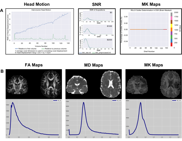
Figure 5: Example Data Metric and Metric QC Histograms. (A) SNR, intervolume head motion, and outlier histograms generated by PyDesigner for the example data downloaded from OpenNeuro. Note that text size has been increased on the plots in this figure for readability. (B) Single subject metric maps histograms of voxel value counts for FA, MD, and MK for the same dataset, visualized through FSLeyes v6.0. Please click here to view a larger version of this figure.
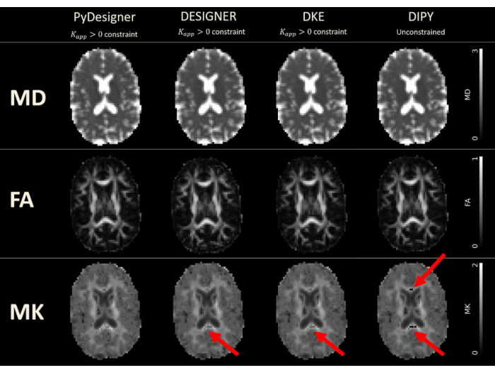
Figure 6: DTI and DKI maps derived from PyDesigner, DESIGNER, DKE, and DIPY. Tensor fitting was performed with Kapp > 0 constraint in PyDesigner, DESIGNER5, and Diffusional Kurtosis Estimator (DKE)27, whereas unconstrained fitting was used in Diffusion Imaging in Python (DIPY)28 due to software limitations. The units for MD are squared micrometers per millisecond (µm2/ms), while the other metrics are dimensionless. Dropouts due to a generic problem from Gibbs ringing correction can be seen in MK maps produced by DESIGNER, DKE, and DIPY. This figure has been reproduced with permission from Dhiman et al.29. Please click here to view a larger version of this figure.
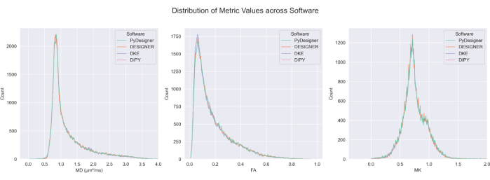
Figure 7: Comparison of FA, MD, and MK across pipelines. The distribution of computed values for FA, MD, and MK from PyDesigner, DESIGNER5, DKE27, and DIPY28 in CSF-excluded brains are similar across most voxels. Metric map calculation across methods is comparable. This figure has been reproduced with permission from Dhiman et al.29. Please click here to view a larger version of this figure.
Discussion
The primary motivation for developing PyDesigner was to implement the key elements of DESIGNER while replacing all MATLAB code with Python, thereby allowing greater portability and accessibility. PyDesigner and DESIGNER Dv1 yield nearly identical outputs29. Nonetheless, there are a few additional options, default settings and minor bug fixes included in PyDesigner. The online PyDesigner documentation16 describes these in detail.
PyDesigner also yields similar results to commonly used Diffusional Kurtosis Estimator (DKE)27 and Diffusion Imaging in Python (DIPY)28 DKI analysis tools29 (see Figure 6 and Figure 7) but the maps generated based on DESIGNER-preprocessed dMRI are considered to be more accurate due to their fitting algorithm as demonstrated by Ades-Aron et al.5. See Figure 6 for a comparison of the MD, FA, and MK metric maps from PyDesigner, DESIGNER5, DKE27, and DIPY28. Figure 7 shows the comparison of MD, FA, and MK histograms from each pipeline. Combining constrained tensor fitting, outlier detection, and apparent kurtosis coefficient correction yields a more robust and accurate tensor fitting, as seen in PyDesigner and DESIGNER5.
An advantage of PyDesigner over DESIGNER Dv1 is that it is available via the NeuroDock Docker container30, which greatly enhances portability and simplifies installation. This container runs across all major OS platforms compatible with Docker, including Windows, Mac OS, and various Linux distributions. Based on user feedback, PyDesigner v2.0 will include updates to the PyDesigner Docker Container. The improvements introduced by the new version of PyDesigner and the introduction of a multi-stage Dockerfile will resolve all existing issues that users are facing. If users have issues with installation, we recommend submitting questions to the PyDesigner discussion page16. Docker's container technology also enables straightforward deployment to high-performance clusters (HPCs) for batch processing DWIs quickly on Docker-compatible local clusters.
PyDesigner also includes microstructural modeling calculations that go beyond DKI, including WMTI3, FBI, and FBWM. For WMTI, a standard DKI dataset is adequate, and the associated microstructural parameters are calculated by default. However, it should be emphasized that the validity of WMTI is restricted to white matter regions with high FA (i.e., FA ≥ 0.4). Some WMTI metrics have limited accuracy due to the assumption of parallel alignment of axons in any given voxel31. FBI32,33,34 is a distinct dMRI method applicable throughout the cerebral white matter, which requires a high b-value (i.e., b ≥ 4000 s/mm2) and dMRI data sampled with a minimum of 64 diffusion encoding directions (along with data for b = 0). The main outputs of FBI are the fiber orientation density function (fODF) for each white matter voxel, which can be used for white matter tractography and serves as an input for FBWM, as well as the intra-axonal fractional anisotropy (FAA). FBWM utilizes the dMRI data from both DKI and FBI to estimate the same parameters as WMTI but with improved accuracy, and it can be applied throughout the white matter regardless of the FA value. Thus, if this additional data is available, then FBWM estimates are preferred over those from WMTI35. As with FBI, FBWM has only been validated in adult cerebral white matter.
In addition to the rotational invariants provided by PyDesigner (RAS orientation), .fib files specific to DSIstudio (LPS orientation) are produced separately for DTI, DKI, and FBI. The .fib files contain ODF directional information for generating tractography profiles for each method. The resulting tractography profiles can be used to generate connectivity matrices at subject and group levels. The DKI and FBI .fib files contain multi-directional information relaying crossing fiber information which is not available with DTI tractography. Moreover, within each .fib file, the various rotational invariants of each method have been included, which can be used in various combinations as criteria for seeding, performing, and stopping the tractography. Further details on DSIstudio can be found on their website36.
Another notable feature of PyDesigner is multi-file input, which allows it to handle various file inputs - NifTi (.nii), compressed NifTi (.nii.gz), DICOM (.dcm), and MRtrix file format (.mif). PyDesigner can automatically identify acquisition information from header metadata regardless of input format and perform corrections accordingly, thereby supporting a hands-off approach. Regardless of differences in protocols, the same command (see above) can be used to process a wide variety of DWIs. This software thus saves time and effort by minimizing manual preprocessing steps and commands. In a recently released update (v1.0-RC10), this has been enhanced by introducing compatibility for multiple echo-time (multi-TE) datasets. This allows PyDesigner to run image preprocessing steps, which are largely independent of TE, on a multi-TE DWI to yield an image with minimal noise and artifacts. TE-dependent tensor calculations are then performed on each TE separately to produce diffusion or kurtosis metrics.
We note that PyDesigner v1.0 does not represent an endpoint in the design of image preprocessing pipelines. The development and validation of image processing tools is an active area of research. In particular, during the preparation of this manuscript, new developments in image denoising and Gibbs ringing removal were proposed, resulting in the release of a revised Designer pipeline, Designer Dv237, that includes improved denoising and correction of Gibbs artifacts for dMRI acquired with Partial Fourier acquisitions35, and is available on the DESIGNER Github38. Likewise, BIDS39 organizational compliance is an important facet of any MRI analysis pipeline. The BIDS format allows for more efficient data sharing and pipeline implementation by establishing a specific set structure for all MRI datatypes. Although PyDesigner is not currently BIDS-compliant, an upcoming version of PyDesigner will include BIDS-compliant outputs. Additionally, PyDesigner was originally written using Python version 3.7. At the time of this publication, Python 3.7 is now considered outdated. However, the information contained in this manuscript is independent of the Python version. That is, the procedures described herein that are important preprocessing functions (e.g., denoising, Gibbs ringing correction, etc.) will follow the same operational and conceptual workflow irrespective of changes in installation procedures. Importantly, as with all Python-based software, future PyDesigner versions will update to a new version of Python. We strive to validate and integrate such developments further over time.
For the most up-to-date version of PyDesigner, including any new documentation relevant to Python version updates, readers are encouraged to consult the website prior to beginning a new analysis and engage in the discussion forum where questions regarding PyDesigner can be submitted16. The Docker implementation for portability is called NeuroDock30, which contains PyDesigner and its dependencies to enable processing across a wide array of platforms.
Disclosures
None.
Acknowledgements
We are grateful for the helpful discussions with Olivia Horn, Daniel Lench, and Graham Warner.
Research reported in this publication was supported, in part, by National Institutes of Health grants R01AG054159, R01AG057602, R01AG055132, R01DC014021, R01NS110347, R21DA050085, F31NS108623, P20GM109040, P50DC000422, T32GM008716, and T32DC014435. The content is solely the responsibility of the authors and does not necessarily represent the official views of the National Institutes of Health. Additional funding was provided by the Litwin Foundation.
Materials
| Name | Company | Catalog Number | Comments |
| Python version 3.7 or above | Python Software Foundation | https://www.python.org/ | |
| FMRIB Software Library (FSL) verison 6.0.2 or above | University of Oxford Centre for Integrative Neuroimaging | https://fsl.fmrib.ox.ac.uk/fsl/fslwiki/ | |
| MRtrix3 version 3.0_RC3 or above | numerous contributors | https://www.mrtrix.org/ | |
| Anaconda | Anaconda | https://anaconda.org/ | |
| Computer | Apple | Mac OS 10.14 | Built on Mac OS 10.14; tested on Mac OS 12.4, Mac OS 13, Windows 11 via WSL |
References
- Jensen, J. H., Helpern, J. A. MRI quantification of non-Gaussian water diffusion by kurtosis analysis. NMR Biomed. 23 (7), 698-710 (2010).
- Basser, P. J. Relationships between diffusion tensor and q-space MRI. Magn Reson Med. 47 (2), 392-397 (2002).
- Fieremans, E., Jensen, J. H., Helpern, J. A. White matter characterization with diffusional kurtosis imaging. Neuroimage. 58 (1), 177-188 (2011).
- Le Bihan, D., Poupon, C., Amadon, A., Lethimonnier, F. Artifacts and pitfalls in diffusion MRI. J Magn Reson Imaging. 24 (3), 478-488 (2006).
- Ades-Aron, B., et al. Evaluation of the accuracy and precision of the diffusion parameter EStImation with Gibbs and NoisE removal pipeline. Neuroimage. 183, 532-543 (2018).
- Veraart, J., Novikov, D. S., Christiaens, D., Ades-aron, B., Sijbers, J., Fieremans, E. Denoising of diffusion MRI using random matrix theory. Neuroimage. 142, 394-406 (2016).
- Kellner, E., Dhital, B., Kiselev, V. G., Reisert, M. Gibbs-ringing artifact removal based on local subvoxel-shifts. Magn Reson Med. 76 (5), 1574-1581 (2016).
- Holland, D., Kuperman, J. M., Dale, A. M. Efficient correction of inhomogeneous static magnetic field-induced distortion in Echo Planar Imaging. Neuroimage. 50 (1), 175-183 (2010).
- Andersson, J. L. R., Sotiropoulos, S. N. An integrated approach to correction for off-resonance effects and subject movement in diffusion MR imaging. Neuroimage. 125, 1063-1078 (2016).
- Godenschweger, F., et al. Motion correction in MRI of the brain. Phys Med Biol. 61 (5), 32-56 (2016).
- Andersson, J. L. R., Graham, M. S., Zsoldos, E., Sotiropoulos, S. N. Incorporating outlier detection and replacement into a non-parametric framework for movement and distortion correction of diffusion MR images. Neuroimage. 141, 556-572 (2016).
- Harris, C. R., et al. Array programming with NumPy. Nature. 585 (7825), 357-362 (2020).
- Virtanen, P., et al. SciPy 1.0: fundamental algorithms for scientific computing in Python. Nat Methods. 17 (3), 261-272 (2020).
- Agrawal, A., Verschueren, R., Diamond, S., Boyd, S. A rewriting system for convex optimization problems. J Control Decis. 5 (1), 42-60 (2018).
- Diamond, S., Boyd, S. CVXPY: A Python-embedded modeling language for convex optimization. , Available from: http://arxiv.org/abs/1603.00943 (2016).
- PyDesigner. , Available from: https://github.com/muscbridge/PyDesigner (2023).
- How to install Linux on Windows with WSL. , Available from: https://learn.microsoft.com/en-us/windows/wsl/install (2023).
- FSL Wiki. , Available from: https://fsl.fmrib.ox.ac.uk/fsl/fslwiki (2024).
- Fsl Instillation. , Available from: https://fsl.fmrib.ox.ac.uk/fsl/fslwiki/FslInstallation/Windows (2024).
- Installing conda. , Available from: https://conda.io/projects/conda/en/stable/user-guide/install/download.html (2024).
- Steps to install Anaconda on Windows Ubuntu terminal. , Available from: https://gist.github.com/kauffmanes/5e74916617f9993bc3479f401dfec7da (2024).
- Install MRtrix3. , Available from: https://www.mrtrix.org (2024).
- PyDesigner Read the Docs. , Available from: https://pydesigner.readthedocs.io/en/latest/ (2024).
- dicomSort. , Available from: https://github.com/muscbridgelab/dicomSort (2024).
- dcm2niix. , Available from: https://github.com/rordenlab/dcm2niix (2024).
- PyDesigner Example Dataset. , Available from: https://openneuro.org/datasets/ds004945 (2024).
- Tabesh, A., Jensen, J. H., Ardekani, B. A., Helpern, J. A. Estimation of tensors and tensor-derived measures in diffusional kurtosis imaging. Magn Reson Med. 65 (3), 823-836 (2011).
- Garyfallidis, E., et al. Dipy, a library for the analysis of diffusion MRI data. Front Neuroinform. 8, 8(2014).
- Dhiman, S., et al. PyDesigner: A Pythonic implementation of the DESIGNER pipeline for diffusion tensor and diffusional Kurtosis imaging. bioRxiv. , (2021).
- Neurodock. , Available from: https://hub.docker.com/r/dmri/neurodock (2024).
- Jelescu, I. O., et al. One diffusion acquisition and different white matter models: How does microstructure change in human early development based on WMTI and NODDI. Neuroimage. 107, 242-256 (2015).
- Jensen, J. H., Russell Glenn, G., Helpern, J. A. Fiber ball imaging. Neuroimage. 124, 824-833 (2016).
- Moss, H. G., Jensen, J. H. High fidelity fiber orientation density functions from fiber ball imaging. NMR Biomed. 35 (1), e4613(2022).
- Moss, H. G., McKinnon, E. T., Glenn, G. R., Helpern, J. A., Jensen, J. H. Optimization of data acquisition and analysis for fiber ball imaging. Neuroimage. 200, 690-703 (2019).
- McKinnon, E. T., Helpern, J. A., Jensen, J. H. Modeling white matter microstructure with fiber ball imaging. Neuroimage. 176, 11-21 (2018).
- DSIstudio. , Available from: https://dsi-studio.labsolver.org (2024).
- Chen, J., et al. Optimization and validation of the DESIGNER dMRI preprocessing pipeline in white matter aging. ArXiv. , arXiv:2305.14445v2 (2024).
- DESIGNER. , Available from: https://github.com/NYU-DiffusionMRI/DESIGNER (2024).
- Gorgolewski, K. J., et al. The brain imaging data structure, a format for organizing and describing outputs of neuroimaging experiments. Sci Data. 3, 160044(2016).
Reprints and Permissions
Request permission to reuse the text or figures of this JoVE article
Request PermissionThis article has been published
Video Coming Soon
Copyright © 2025 MyJoVE Corporation. All rights reserved