Brain Infarct Segmentation and Registration on MRI or CT for Lesion-symptom Mapping

Podsumowanie

Provided here is a practical tutorial for an open-access, standardized image processing pipeline for the purpose of lesion-symptom mapping. A step-by-step walkthrough is provided for each processing step, from manual infarct segmentation on CT/MRI to subsequent registration to standard space, along with practical recommendations and illustrations with exemplary cases.

Streszczenie

In lesion-symptom mapping (LSM), brain function is inferred by relating the location of acquired brain lesions to behavioral or cognitive symptoms in a group of patients. With recent advances in brain imaging and image processing, LSM has become a popular tool in cognitive neuroscience. LSM can provide fundamental insights into the functional architecture of the human brain for a variety of cognitive and non-cognitive functions. A crucial step in performing LSM studies is the segmentation of lesions on brains scans of a large group of patients and registration of each scan to a common stereotaxic space (also called standard space or a standardized brain template). Described here is an open-access, standardized method for infarct segmentation and registration for the purpose of LSM, as well as a detailed and hands-on walkthrough based on exemplary cases. A comprehensive tutorial for the manual segmentation of brain infarcts on CT scans and DWI or FLAIR MRI sequences is provided, including criteria for infarct identification and pitfalls for different scan types. The registration software provides multiple registration schemes that can be used for processing of CT and MRI data with heterogeneous acquisition parameters. A tutorial on using this registration software and performing visual quality checks and manual corrections (which are needed in some cases) is provided. This approach provides researchers with a framework for the entire process of brain image processing required to perform an LSM study, from gathering of the data to final quality checks of the results.

Wprowadzenie

Lesion-symptom mapping (LSM), also called lesion-behavior mapping, is an important tool for studying the functional architecture of the human brain¹. In lesion studies, brain function is inferred and localized by studying patients with acquired brain lesions. The first case studies linking neurological symptoms to specific brain locations performed in the nineteenth century already provided fundamental insights into the anatomical correlates of language and several other cognitive processes². Yet, the neuroanatomical correlates of many aspects of cognition and other brain functions remained elusive. In the past decades, improved structural brain imaging methods and technical advances have enabled large-scale in vivo LSM studies with high spatial resolution (i.e., at the level of individual voxels or specific cortical/subcortical regions of interest)^1,2. With these methodological advances, LSM has become an increasingly popular method in cognitive neuroscience and continues to offer new insights into the neuroanatomy of cognition and neurological symptoms³. A crucial step in any LSM study is the accurate segmentation of lesions and registration to a brain template. However, a comprehensive tutorial for the preprocessing of brain imaging data for the purpose of LSM is lacking.

Provided here is a complete tutorial for a standardized lesion segmentation and registration method. This method provides researchers with a pipeline for standardized brain image processing and an overview of potential pitfalls that must be avoided. The presented image processing pipeline was developed through international collaborations⁴ and is part of the framework of the recently founded Meta VCI map consortium, whose purpose is performing multicenter lesion-symptom mapping studies in vascular cognitive impairment <www.metavcimap.org>⁵. This method has been designed to process both CT and MRI scans from multiple vendors and heterogeneous scan protocols to allow combined processing of imaging datasets from different sources. The required RegLSM software and all other software needed for this protocol is freely available except for MATLAB, which requires a license. This tutorial focuses on the segmentation and registration of brain infarcts, but this image processing pipeline can also be used for other lesions, such as white matter hyperintensities⁶.

Prior to initiating an LSM study, a basic understanding of the general concepts and pitfalls is required. Several detailed guidelines and a hitchhiker's guide are available^1,3,6. However, these reviews do not provide a detailed hands-on tutorial for the practical steps involved in gathering and converting brain scans to a proper format, segmenting the brain infarct, and registering the scans to a brain template. The present paper provides such a tutorial. General concepts of LSM are provided in the introduction with references for further reading on the subject.

General aim of lesion-symptom mapping studies

From the perspective of cognitive neuropsychology, brain injury can be used as a model condition to better understand the neuronal underpinnings of certain cognitive processes and to obtain a more complete picture of the cognitive architecture of the brain¹. This is a classic approach in neuropsychology that was first applied in post-mortem studies in the nineteenth century by pioneers like Broca and Wernicke². In the era of functional brain imaging, the lesion approach has remained a crucial tool in neuroscience because it provides proof that lesions in a specific brain region disrupt task performance, while functional imaging studies demonstrate brain regions that are activated during the task performance. As such, these approaches provide complementary information¹.

From the perspective of clinical neurology, LSM studies can clarify the relationship between the lesion location and cognitive functioning in patients with acute symptomatic infarcts, white matter hyperintensities, lacunes, or other lesion types (e.g., tumors). Recent studies have shown that such lesions in strategic brain regions are more relevant in explaining cognitive performance than global lesion burden^2,5,7,8. This approach has the potential to improve understanding of the pathophysiology of complex disorders (in this example, vascular cognitive impairment) and may provide opportunities for developing new diagnostic and prognostic tools or supporting treatment strategies².

LSM also has applications beyond the field of cognition. In fact, any variable can be related to lesion location, including clinical symptoms, biomarkers, and functional outcome. For example, a recent study determined infarct locations that were predictive of functional outcome after ischemic stroke¹⁰.

Voxel-based versus region of interest-based lesion-symptom mapping

To perform lesion-symptom mapping, lesions need to be segmented and registered to a brain template. During the registration procedure, each patient's brain is spatially aligned (i.e., normalized or registered to a common template) to correct for differences in brain size, shape, and orientation so that each voxel in the lesion map represents the same anatomical structure for all patients⁷. In standard space, several types of analyses can be performed, which are briefly summarized here.

A crude lesion-subtraction analysis can be performed to show the difference in lesion distribution in patients with deficits compared to patients without deficits. The resulting subtraction map show regions that are more often damaged in patients with deficits and spared in patients without deficits¹. Though a lesion-subtraction analysis can provide some insights into correlates of a specific function, it provides no statistical proof and is now mostly used when the sample size is too low to provide enough statistical power for voxel-based lesion-symptom mapping.

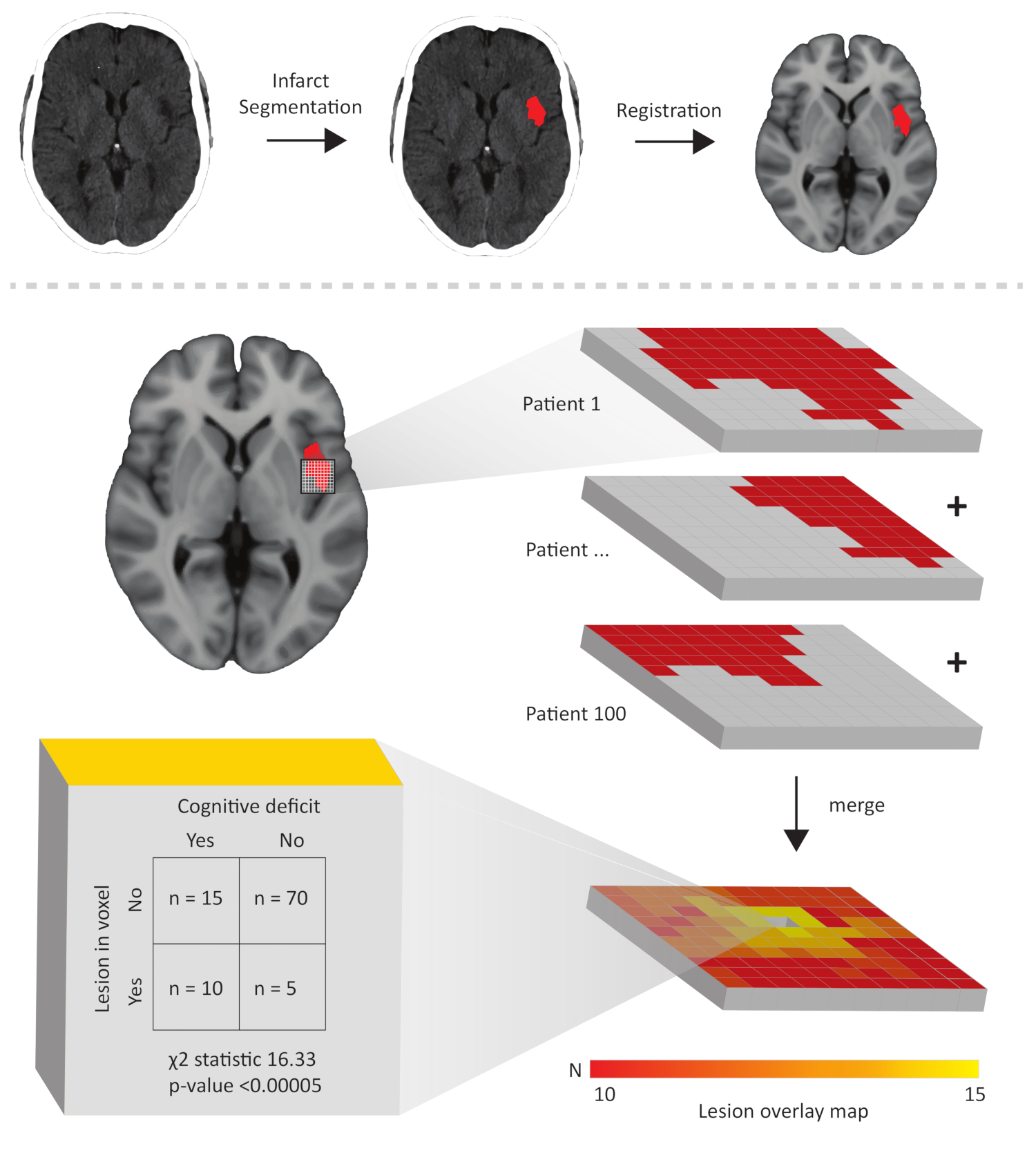
In voxel-based lesion-symptom mapping, an association between the presence of a lesion and cognitive performance is determined at the level of each individual voxel in the brain (Figure 1). The main advantage of this method is the high spatial resolution. Traditionally, these analyses have been performed in a mass-univariate approach, which warrants correction for multiple testing and introduces a spatial bias caused by inter-voxel correlations that are not taken into account^1,10,11. Recently developed approaches that do take inter-voxel correlations into account (usually referred to as multivariate lesion-symptom mapping methods, such as Bayesian analysis¹³, support vector regression^4,14, or other machine learning algorithms¹⁵) show promising results and appear to improve the sensitivity and specificity of findings from voxel-wise LSM analyses compared to traditional methods. Further improvement and validation of multivariate methods for voxel-wise LSM is an ongoing process. The best method choice for specific lesion-symptom mapping depends on many factors, including the distribution of lesions, outcome variable, and underlying statistical assumptions of the methods.

In the region of interest (ROI)-based lesion-symptom mapping, an association between the lesion burden within a specific brain region and cognitive performance is determined (see Figure 1 in Biesbroek et al.² for an illustration). The main advantage of this method is that it considers the cumulative lesion burden within an anatomical structure, which in some cases may be more informative than a lesion in a single voxel. On the other hand, ROI-based analyses have limited power for detecting patterns that are only present in a subset of voxels in the region¹⁶. Traditionally, ROI-based lesion-symptom mapping is performed using logistic or linear regression. Recently, multivariate methods that deal better with collinearity have been introduced (e.g., Bayesian network analysis¹⁷, support vector regression^4,18, or other machine learning algorithms¹⁹), which may improve the specificity of findings from lesion-symptom mapping studies.

Patient selection

In LSM studies, patients are usually selected based on a specific lesion type (e.g., brain infarcts or white matter hyperintensities) and the time interval between diagnosis and neuropsychological assessment (e.g., acute vs. chronic stroke). The optimal study design depends on the research question. For example, when studying the functional architecture of the human brain, acute stroke patients are ideally included because functional reorganization has not yet occurred in this stage, whereas chronic stroke patients should be included when studying the long-term effects of stroke on cognition. A detailed description of considerations and pitfalls in patient selection is provided elsewhere⁷.

Brain image preprocessing for the purpose of lesion-symptom mapping

Accurate lesion segmentation and registration to a common brain template are crucial steps in lesion-symptom mapping. Manual segmentation of lesions remains the gold standard for many lesion types, including infarcts⁷. Provided is a detailed tutorial on criteria for manual infarct segmentation on CT scans, diffusion weighted imaging (DWI), and fluid-attenuated inversion recovery (FLAIR) MRI sequences in both acute and chronic stages. The segmented infarcts (i.e., the 3D binary lesion maps) need to be registered before any across-subject analyses are performed. This protocol uses the registration method RegLSM, which was developed in a multicenter setting⁴. RegLSM applies linear and non-linear registration algorithms based on elastix²⁰ for both CT and MRI, with an additional CT processing step specifically designed to enhance registration quality of CT scans²¹. Furthermore, RegLSM allows for using different target brain templates and an (optional) intermediate registration step to an age-specific CT/MRI template²². The possibility of processing both CT and MRI scans and its customizability regarding intermediate and target brain templates makes RegLSM a highly suitable image processing tool for LSM. The entire process of preparing and segmenting CT/MRI scans, registration to a brain template, and manual corrections (if required) are described in the next section.

Figure 1: Schematic illustration of the concept of voxel-based lesion-symptom mapping. The upper part shows the brain image pre-processing steps consisting of segmenting the lesion (an acute infarct in this case) followed by registration to a brain template (the MNI-152 template in this case). Below, a part of the registered binary lesion map of the same patient is shown as a 3D grid, where each cube represents a voxel. Taken together with the lesion maps of 99 other patients, a lesion overlay map is generated. For each voxel, a statistical test is performed to determine the association between lesion status and cognitive performance. The chi-squared test shown here is just an example, any statistical test could be used. Typically, hundreds of thousands of voxels are tested throughout the brain, followed by a correction for multiple comparisons. Please click here to view a larger version of this figure.

Protokół

This protocol follows the guidelines of our institutions human research ethics committee.

1. Collection of Scans and Clinical Data

1. Collect brain CT or MRI scans of patients with ischemic stroke. Most scanners save the scans as DICOM (Digital Imaging and Communications in Medicine) files that can be copied to a hard disk or server.
   NOTE: Scans from every scanner type, scan protocol, and MRI field strength can be used, as long as 1) the time window requirements for the used scan type are met (see Table 1) and 2) there are no artifacts that hamper accurate infarct delineation. A detailed tutorial on artifact detection on CT and MRI is provided elsewhere^23,24. An example of commonly occurring motion artifacts on CT is provided in Figure 2, and examples of scans of good quality are provided in the exemplar cases in the results section. Infarcts can be segmented on scans with any slice thickness and any in-plane image resolution. However, thin slices and high in-plane resolution will enable a more accurate representation of the infarct to the brain template.
2. Collect the clinical variables in a data file (e.g., Excel) by making separate rows for each case and columns for each clinical variable. For infarct segmentation, include at least the variables date of stroke and date of imaging or a variable that indicates the time interval between stroke and imaging.
3. Ensure that ethical guidelines and regulations regarding privacy are followed. Ensure that the data is either anonymized or coded. Pay specific attention to the removal of patient data such as name, address, and date of birth that are stored in the DICOM files as tags. These tags can be cleared using dcm2niix (free download available at <https://github.com/rordenlab/dcm2niix>)²⁵.

2. Conversion of DICOM Images to Nifti Files

1. To convert the DICOM images to uncompressed nifti files using the dcm2niix tool, type "[folder path of dcm2niix.exe]\dcm2niix %d_%p [folder path of dicom files]" in the command prompt. An example of the command with the folders paths inserted could be C:\users\matthijs\dcm2niix %d_%p C:\users\matthijs\dicom\. This command will run the dcm2niix executable, convert the DICOM images in the selected folder and save the nifti files in the same folder.
   NOTE: The addition %d_%p ensures that the series description and protocol name are inserted in the file name. Additional features including options for batch conversion are provided in the dcm2niix manual at <https://www.nitrc.org/plugins/mwiki/index.php/dcm2nii:MainPage>. Other open source tools can be used for the conversion of DICOM images to nifti files, as well.
2. Ensure that the name of the scan type (CT, FLAIR, DWI, or other sequence names) is copied into the file name during conversion (this option is available in dcm2niix).
3. For MRI scans, select DWI or FLAIR sequences for segmentation. Alternatively, any other structural sequence on which the infarct is visible can be used. See Table 1 for appropriate time windows after stroke in which CT, DWI, or FLAIR can be used for infarct segmentation.
4. Organize the nifti files in a convenient folder structure with a subfolder for each case (see the manual of RegLSM and Supplementary Figure 1). This manual can be downloaded from <www.metavcimap.org/support/software-tools>.
   NOTE: This folder structure is a requirement for the registration software RegLSM (see section 4). An update of RegLSM, making it BIDS (brain imaging data structure²⁶, see <http://bids.neuroimaging.io>) compatible, is currently being developed and will soon be released.

3. Infarct Segmentation

1. General remarks applying to all scan types
   1. Ensure that the person who performs and evaluates segmentation and registration is blinded to the outcome variable (usually a cognitive measure) to avoid bias.
   2. Note that infarcts are usually segmented on transversal slices, but segmentation can be performed in any slice orientation.
   3. Ensure ideal viewing conditions during infarct segmentation by using a high-resolution monitor display and optimal ambient light to provide a comfortable setting. Manually adjust the image contrast during segmentation to provide optimal contrast between healthy brain tissue. Be consistent in applying similar settings across subjects.
2. Infarct segmentation on CT
   1. First check whether the scan was performed at least 24 h after stroke symptom onset. Within 24 h, the acute infarct is not or only partially visible on CT and the scan cannot be used for segmentation⁷. See Figure 3 for an illustration.
   2. Open the native CT using ITK-SNAP software (free download available at <www.itksnap.org>)²⁷. In ITK-SNAP, click File | open main image from the dropdown menu. Click browse and select the file to open the scan. If the default contrast setting provides poor contrast between healthy brain tissue and the lesion, adjust the contrast settings. To do so, click Tools | image contrast | contrast adjustment.
      NOTE: Any open source software can also be used.
   3. If available, open a CT that was performed within 24 h after stroke symptom onset in a separate instance as the reference to distinguish the acute infarct from old ischemic lesions such as lacunes, (sub)cortical infarcts, or white matter hyperintensities.
   4. Identify the infarct based on the following characteristics. Infarcts have a low signal (i.e., hypodense) compared to normal brain tissue.
      1. In the acute stage (first weeks), large infarcts can cause mass effect resulting in displacement of surrounding tissues, compression of ventricles, midline shift and obliteration of sulci. There can be hemorrhagic transformation which is visible as regions with high signal (i.e. hyperdens) within the infarct.
      2. In the chronic stage (months to years), the infarct will consist of a hypodens cavitated center (with a similar density as the cerebrospinal fluid) and a less hypodense rim which represents damaged brain tissue. Both the cavitated center and hypodens rim must be segmented as infarct. In case of large infarct, there can be ex vacuo enlargement of adjacent sulci or ventricles.
         NOTE: Tissue displacement due to mass effect or ex vacuo enlargement of structures should not be corrected for during segmentation (i.e., only the full extent of the infarct has to be segmented). Correction for tissue displacement takes place during the registration and subsequent steps.
   5. Segment the infarcted brain tissue using the paintbrush mode from the main toolbar (left-click to draw, right-click to erase). Alternatively, use the polygon mode to place anchor points at the borders of the lesion (these points are automatically connected with lines) or hold the left mouse button while moving the mouse over the borders of the lesion. Once all anchor points are connected, click accept to fill the delineated area.
   6. Avoid the fogging phase, which refers to the phase in which the infarct becomes isodense on CT (which co-occurs with infiltration of the infarcted tissue with phagocytes). This typically occurs 14-21 days after stroke onset, but in rare cases can occur even earlier²⁸. During this period, the infarct can become invisible or its boundaries become less clear, making this stage unsuitable for infarct segmentation. After the fogging phase, the lesion becomes hypodense again when cavitation and gliosis occur. See Figure 4 for two examples.
   7. After finishing the segmentation, save it as a binary nifti file in the same folder as the scan by clicking segmentation | save segmentation image from the dropdown menu, then save the segmentation by giving it the exact same name as the segmented scan, with the extension of .lesion (e.g., if the scan was saved as "ID001.CT.nii", save the segmentation as "ID001.CT.lesion.nii").
3. Infarct segmentation on DWI
   1. First check if the DWI was performed within 7 days of stroke onset. Infarcts are visible on DWI within several hours after stroke onset and their visibility on DWI gradually decreases after approximately 7 days (see paragraph 2 in the discussion for more details).
   2. Open the DWI in ITK-SNAP (in the same way as done in step 3.2.2).
      NOTE: A DWI sequence generates at least two images for most scan protocols, one with a b-value = 0, which is a standard T2-weighted image, and one with a higher b-value, which is the scan that captures the actual diffusion properties of the tissue. The higher the b-value, the stronger the diffusion effects. For ischemic stroke detection, a b-value around 1000 s/mm² is often used, as this provides a good contrast-to-noise ratio in most cases²⁹. The image with a high b-value is used for infarct segmentation.
   3. Open the apparent diffusion coefficient (ADC) sequence in a separate instance of ITK-SNAP for reference.
   4. Identify and annotate the infarcted brain tissue based on the high signal (i.e., hyperintense) on DWI and low signal (i.e., hypointense) on the ADC (see Figure 5). ADC values in the infarct gradually increase until ADC normalizes on average 1 week after the stroke³⁰, but in some cases, the ADC may already be (nearly) normalized after several days if there is much vasogenic edema.
      NOTE: In DWI images with low b-values, brain lesions with an intrinsic high T2 signal (such as white matter hyperintensities) can also appear hyperintense. This phenomenon is called T2 shine-through³¹. However, with increasing b-values, this phenomenon becomes less relevant, as the signal on the DWI image more strongly reflects diffusion properties instead of intrinsic T2 signal. With modern DWI scan protocols (usually with b-value=1000 or higher), the T2 shine-through effects are limited³².
   5. Do not mistake a high DWI signal near interfaces between air and either tissue or bone, which are a commonly observed artifact, for an infarct. See Figure 5.
   6. Save the annotation as a binary nifti file, giving it the exact same name as the segmented scan, with the extension of .lesion (in the same way as done in step 3.2.7).
4. Infarct segmentation on FLAIR
   1. First, check if the scan was performed >48 h after stroke symptom onset. In the hyperacute stage, the infarct is usually not visible on the FLAIR sequence or the exact boundaries of the infarct are unclear³¹ (see Figure 6).
   2. Open the FLAIR in ITK-SNAP in the same way as done in step 3.2.2.
   3. Open the T1 a separate instance of ITK-SNAP for reference, if available.
   4. Identify and segment the infarcted brain tissue based on the following characteristics.
      1. In the acute stage (first few weeks), the infarct is visible as a more or less homogeneous hyperintense lesion, with or without apparent swelling and mass effect (Figure 5).
      2. In the chronic stage (months to years), the infarct is cavitated, meaning the center becomes hypo- or isointense on FLAIR. This cavity can be most accurately identified on the T1. In most cases, the cavitated center is surrounded by a hyperintense rim on the FLAIR, representing gliosis.³³.
         NOTE: However, there is a considerable amount of variation in the degree of cavitation and gliosis of chronic infarcts. Segment both the cavity and the hyperintense rim as infarcts (see step 3.2.5). A FLAIR hyperintense lesion is not always an infarct. In the acute stage, small subcortical infarcts can easily be distinguished from white matter hyperintensities or other chronic lesions such as lacunes of presumed vascular origin when there is a DWI available (see Figure 5). In the chronic stage, it can be more difficult. See paragraph 3 in the discussion for more information on how to discriminate these lesion types in the chronic stage.
   5. Save the annotation as a binary nifti file, giving it the exact same name as the segmented scan, with the extension of .lesion (in the same way as done in step 3.2.7).

Scan type	Time window after stroke	Infarct properties	Reference scan	Pitfalls
CT	>24 h	Acute: hypodense	-	- Fogging phase
		Chronic: hypodense cavity with CSF and less hypodense rim		- Hemorrhagic transformation
DWI	<7 days	Hyperintense	ADC: typically hypointense	- T2 shinethrough
				- High DWI signal near interfaces between air and bone/tissue
FLAIR	>48 h	Acute: hyperintense	Acute: DWI/ADC, T1 (isointense or hypointense)	- White matter hyperintensities
		Chronic: hypointense or isointense (cavity), hyperintense rim	Chronic: T1 (hypointense cavity with CSF characteristics).	- Lacunes

Table 1: Summary of criteria for infarct segmentation for different scan types.

4. Registration to Standard Space

1. Download RegLSM from <www.metavcimap.org/features/software-tools>⁴. Use this tool to process CT scans and any kind of MRI sequence. The registration procedure is illustrated in Figure 7.
   NOTE: Optional features in RegLSM include registration to an intermediate CT/MRI template that more closely resembles the scans of older patients with brain atrophy²². By default, the CT and MRI scan are registered to the MNI-152 template³⁴, but this can be replaced by other templates if this better suits the study. Different registration schemes are illustrated in Figure 7. Other open source registration tools can also be used for this step.
2. Check 1) if the nifti files are not compressed, 2) that the file name of the segmented scan contains the term CT, FLAIR, or DWI, and 3) that the file name of the lesion annotation contains the same term with an appended ".lesion". If these first three steps are followed, the data is fully prepared for registration and nothing needs to be changed.
3. Open MATLAB (version 2015a or higher), set the current folder to RegLSM (this folder can be downloaded from ³⁵ (version 12 or higher, free download at <https://www.fil.ion.ucl.ac.uk/spm/>) by typing addpath {folder name of SPM}. Next, type RegLSM to open the GUI.
4. Select test mode in the registration dropdown menu to perform the registration for a single case. In the test mode panel, select the scan (CT, FLAIR, or DWI), annotation, and optionally the T1, using the open image button. Select the registration scheme: CT, FLAIR with or without T1, DWI with or without T1.
5. Alternatively, select batch mode to register the scans of all cases in the selected folder in batch mode.
6. Ensure that RegLSM saves the resulting registration parameters and the registered scans (including intermediate steps) and the registered lesion map in subfolders that are automatically generated. During this process, the registered scans and lesion maps are resampled to match the resolution (isotropic 1 mm³ voxels) and angulation of the MNI-152 template.

5. Review Registration Results

1. Select the option check results in the RegLSM GUI and browse to the main folder with the registration results. The GUI will automatically select the registered scan with the registered lesion map, and the MNI-152 template with the registered lesion map in transverse, sagittal, and coronal orientations (see Figure 8).
2. Scroll through the registered scan and use the crosshair to check the alignment of the registered scan and the MNI-152 template. Pay specific attention to the alignment of recognizable anatomical landmarks such as the basal ganglia, ventricles, and skull.
3. Mark all failed registrations in a separate column in the data file (made in step 1.2) for the subsequent manual correction in section 6.
   NOTE: Common errors in the registration are imperfect alignment due to the mass effect caused by the lesion in the acute stage, or ex vacuo enlargement of ventricles in the chronic stage. See Figure 3 and Figure 5 for examples of such misalignment. Another common error is a misalignment of the tentorium cerebelli, in which case an occipital infarct can overlap with the cerebellum in the template. Misalignment of tissues that are not lesioned is not an issue when only the binary lesion maps are used in the subsequent lesion-symptom mapping analyses. In such cases, only the lesions need to be perfectly aligned.

6. Manually Correct Registration Errors

1. For the lesion maps that need correction, open the MNI-152 T1 template in ITK-SNAP and select from the segmentation menu | open segmentation | registered lesion map, which is now overlaid on the template.
2. Open the registered brain scan in a separate instance of ITK-SNAP for reference.
3. Correct the registered lesion map in ITK-SNAP for any type of misalignment that is mentioned in step 5.3 using the brush function to add voxels (left click) or remove voxels (right click). Carefully compare the registered scan and overlaid lesion map (see step 5.2) with the MNI-152 template and overlaid lesion map in ITK-SNAP (see step 6.1) to identify the regions of misalignment. See Figure 3 and Figure 5.
4. After manually correcting lesion map in MNI space, perform a final check by comparing the segmented native scan of the patient with the corrected lesion map in MNI space (i.e., the results of step 6.3). Ensure that the corrected lesion map in MNI space now accurately represents the infarct in native space. Pay specific attention to the recognizable landmarks such as basal ganglia, ventricles, and skull (similar to step 5.2).
5. Save the corrected lesion map in MNI space as a binary nifti file in the same folder as the uncorrected lesion map in MNI-152 space, giving it the exact same name as the uncorrected lesion map, with the extension of .corrected.

7. Preparing Data for Lesion-symptom Mapping

1. Rename all the lesion maps. By default, RegLSM saved the lesion maps in a subfolder with the file name "results". Include the subject ID in the file name. In the case of manual correction, be sure to select and rename the corrected file.
2. Copy all the lesion maps into a single folder.
3. Perform a sanity check of the data by randomly selecting and inspecting several lesion maps in ITK-SNAP and compare these with the native scans to rule out systematic errors in data processing such as left-right flipping.
4. Use MRIcron <https://www.nitrc.org/projects/mricron> to perform another sanity check of the data by creating a lesion overlap image to check if no lesions are located outside the brain template. Do this by selecting the draw dropdown menu | statistics | create overlap images.
   NOTE: The resulting lesion overlay map can be projected on the MNI-152 template and inspected using, for example, MRIcron or ITK-SNAP.
5. The lesion maps are now ready to be used for voxel-based lesion-symptom mapping or for calculation of infarct volumes within specific regions of interest using an atlas that is registered to the same standard space as the lesion maps (in this case, MNI-152 space for which many atlases are available, only a few of which are cited below^36,37,38).

Wyniki

Exemplar cases of brain infarct segmentations on CT (Figure 3), DWI (Figure 5), and FLAIR (Figure 6) images, and subsequent registration to the MNI-152 template are provided here. The registration results shown in Figure 3B and Figure 5C were not entirely successful, as there was misalignment near the frontal horn of the ventricle. The regis...

Dyskusje

LSM is a powerful tool to study the functional architecture of the human brain. A crucial step in any lesion-symptom mapping study is the preprocessing of imaging data, segmentation of the lesion and registration to a brain template. Here, we report a standardized pipeline for lesion segmentation and registration for the purpose of lesion-symptom mapping. This method can be performed with freely available image processing tools, can be used to process both CT and structural MRI scans, and covers the entire process of pre...

Materiały

Name	Company	Catalog Number	Comments
dcm2niix	N/A	N/A	free download https://github.com/rordenlab/dcm2niix
ITK-SNAP	N/A	N/A	free download www.itksnap.org
MATLAB	MathWorks	N/A	Version 2015a or higher
MRIcron	N/A	N/A	free download https://www.nitrc.org/projects/mricron
RegLSM	N/A	N/A	free download www.metavcimap.org/support/software-tools
SPM12b	N/A	N/A	free download https://www.fil.ion.ucl.ac.uk/spm/