
0:00
Overview
1:22
Principles of HPLC
5:05
Preparation of the Mobile Phase
6:08
Preparation of Component and Standard Solutions
7:25
HPLC Setup
9:25
Diet Soda Samples
10:16
Results
11:27
Applications
12:44
Summary
高性能液相色谱法 (HPLC)
资料来源: 博士保罗 · 鲍尔-普渡大学
高性能液相色谱法 (HPLC) 是重要的分析方法,通常用来分离和量化的液体样品的组件。在这种技术,通过一列与绑定到表面的第二个阶段包含小多孔颗粒包装抽解决方案 (第一阶段)。不同溶解度的两个阶段中的示例组件导致组件移动的列具有不同的平均速度,从而创造这些组分的分离。泵送的解决方案被称为流动相,而列的阶段称为固定相。
有几种模式的液相色谱法,取决于采用的固定和/或移动相的类型。本实验使用反相色谱固定相是非极性,极性流动相。固定相用于是保税区向 3 µ m 二氧化硅颗粒,流动相时缓冲溶液与极性的有机改性 (乙腈) 添加到其洗脱强度会发生变化的 C18 烃族组成。在此窗体,硅可以用于样品是水溶性的提供一系列广泛的应用。在这个实验中,经常发现在减肥软饮料 (即咖啡因、 苯甲酸,阿斯巴甜) 的三个组成部分的混合物分离了。七准备的解决方案包含三个物种已知的量使用,然后记录他们的图谱。
在高效液相色谱法实验,高压泵从水库通过喷油器采取流动相。然后,它流经反相 C18 填充柱的组分分离。最后,流动相进入检测器细胞,吸光度按 220 nm 和废瓶中的结束。组件从进样口到探测器旅行所花费的时间量称为保留时间。
液相色谱分析法用在这个实验中,分离执行反相柱上的位置。列尺寸是 3 毫米 (身份证) x 100 毫米和白炭黑包装 (3 微米粒子大小) 羧基化填充剂测分配 C18 (ODS)。Rheodyne 6 端口旋转注射阀用于最初存储在一个小的循环中的样品和样品引入移动阶段后,旋转阀。
检测是通过吸收光谱在波长为 220 nm。这个实验可以运行在 254 nm,如果探测器不是变量。从探测器的数据具有模拟电压输出,这衡量使用数字多用表 (DMM),并且通过与数据采集程序加载计算机读取。由此产生的色谱样品中有一个为每个组件的高峰。对于这个实验,所有三个组件洗脱在 5 分钟以内。
本实验使用一个单一的流动相和泵,称为等度流动相。很难分离的样品,可以用于梯度的流动相。这是当初始流动相是主要是一个水,和随着时间推移,第二有机流动相逐渐添加到整体流动相。随着时间推移,这降低了组件保留次数和工作方式类似于温度梯度对气相色谱仪,此方法引发此相的极性。有某些情况下,列加热 (通常到 40 ° C),其中带走任何保留时间与环境温度的变化相关的错误。
在反相高效液相色谱法,列固定相填料通常 C4,C8 或 C18 填料。C4 列是主要为大分子量的蛋白质,而 C18 柱是肽和低分子量的基本示例。
吸收光谱法检测是选择的压倒性的检测方法,吸收光谱的组件都是选择的唾手可得的。一些系统使用电化学测量,如电导率或碳纤,作为他们的检测方法。
对于这个实验,流动相是主要 20%乙腈和 80%纯化 (DI) 去离子的水。加少量的醋酸降低流动相,硅在固定包装阶段保持不离州的 ph 值。这减少了吸附峰从尾矿,给窄峰。然后,ph 值被调整与 40%氢氧化钠提高 ph 值,帮助减少组分的保留时间。
每个组使用一套 7 小瓶含有不同浓度的标准溶液 (表 1)。第一 3 用于标识每个峰,和最后的 4 个用于创建为每个组件的校准图表。标准 1-3 还用于校准图表。
| 数量 | 咖啡因 (毫升) | 苯甲酸 (毫升) | 阿斯巴甜 (毫升) |
| 1 | 4 | 0 | 0 |
| 2 | 0 | 4 | 0 |
| 3 | 0 | 0 | 4 |
| 4 | 1 | 1 | 1 |
| 5 | 2 | 2 | 2 |
| 6 | 3 | 3 | 3 |
| 7 | 5 | 5 | 5 |
表 1。用于准备 7 提供的工作标准 (每一个标准的总容量是 50 毫升) 的股票标准卷。
1.使流动相
- 准备到大约 1.5 L 的纯净 DI 水加入 400 毫升的乙腈的流动相。
- 仔细地将 2.4 毫升冰醋酸的添加到此解决方案。
- 稀溶液到容量瓶用纯净的 DI 水 2.0 L 总体积。生成的解决方案应该有 2.8 到 3.2 之间的 ph 值。
- 通过添加 40%氢氧化钠,落与校准数字 pH 计使用调整其 ph 值至 4.2。当 ph 值达到 4.0 中慢慢加入。这应采取约 50 滴来完成。
- 通过真空脱气的解决方案,以消除可能堵塞色谱柱的固体 0.47 µ m 尼龙 66 膜过滤器过滤流动相。它是重要脱气流动相以避免泡沫,这可以导致空虚在固定相在列的入口处或其方式工作探测器单元格中,用紫外吸光度造成不稳定。
2.创建组件解决方案
需要进行的三个组成部分是咖啡因 (0.8 毫克/毫升)、 苯甲酸钾 (1.4 毫克/毫升) 和阿斯巴甜 (L-天冬氨酸-L-苯丙氨酸甲酯) (6.0 毫克/毫升)。这些浓度,一次稀释以同样的方式,把标准放在苏打水样本中发现的水平。
- 0.40 g 的咖啡因添加 500 毫升容量瓶里,然后稀释至 500 毫升马克用去离子水。
- 添加苯甲酸的 0.70 g 到 500 毫升的容量瓶,然后稀释至 500 毫升马克用去离子水。
- 阿斯巴甜 0.60 g 添加 100 毫升容量瓶里,然后稀释至 100 毫升马克用去离子水。将此解决方案放在冰箱里,避免贮藏过程中的分解。
3.使 7 标准的解决方案
三个要素都有不同的分配系数,从而影响每个如何与两个阶段进行交互。分配系数越大,更多的时间,该组件花费在固定相,导致更长的保留时代在到达探测器。
- 以下表 1,吸管适量的每个组件到 50 毫升容量瓶中的图表。
- 稀释每个股票的解决方案 50 毫升上的标志与流动相的容量瓶。
- 每个标准溶液倒入标记的小瓶,在样品架上。
- 在冰箱里,以及 50 毫升的容量瓶中的剩余解决方案存储样品的架。
4.检测高效液相色谱系统的初始设置
- 确认废线是废物容器中,并没有回收回流动相。
- 验证的流动相流速设置为 0.5 m l/min。这是高得足以让所有的山峰在 5 分钟内洗脱和很慢的速度,以便好决议。
- 验证的最小值和最大的压力和流量都设置为溶剂输送系统 (泵) 的前面板上的正确值。
- 最小压力值设置: 250 psi (这是为了关闭泵,如果发生了泄漏)。
- 最大压力设置: 4,000 psi (这是为了保护泵免于破碎,如果堵塞形式)。
- 按"零"探测器的前面板上设置的空白 (空白是纯流动相)。
- 冲洗用去离子水,然后用几个卷的工作标准,以分析,和注射器吸满该解决方案之一的 100 µ L 注射器。从开始 3 单组分样品,它允许识别感兴趣的每个部件的高峰期。
5.手动注射样品和数据收集
- 与荷载作用位置的注射器手柄,慢慢注入 100 μ L 的解决方案通过隔膜端口。
- 验证数据采集程序被设置为收集数据为 300 s,允许足够的时间让所有 3 个波峰通过探测器洗脱。
- 当准备好开始审判时,旋转的插入位置 (样品注入流动相) 的喷油器句柄,然后单击"开始审判"计算机数据采集程序立即。标准 1-3,唯一的三序贯峰出现在屏幕上 (图 1) 运行期间。
- 一次 300 s 已通过,数据收集发送提示保存的数据文件。保存的数据在下一个合适的文件名称 (例如,性病 #1)。
- 注意到以秒为单位为每项试验,在确定该组件使用的高峰时间。
- 从鼻中隔删除注射器,为每个剩余的工作标准,使用每个色谱确定从第一次运行的同一时间重复此过程。
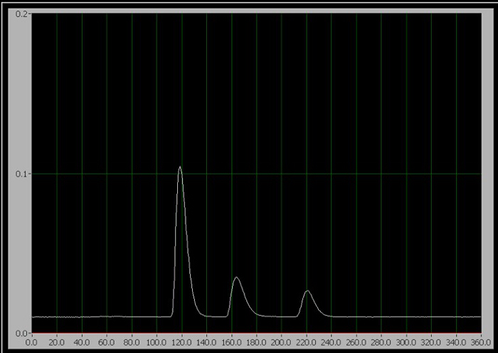
图 1。3 组件层析图谱。从左到右,他们是咖啡因、 阿斯巴甜和苯甲酸。
6.样品的减肥苏打水
健怡可乐、 百事轻怡、 零度可乐是"未知"。他们有被冷落在打开容器一夜之间摆脱碳化,泡沫是不好的高效液相色谱系统。这足以摆脱任何气体样品中。
- 约 2 毫升的无糖苏打水引入塑料注射器。
- 通过扭曲它到位的过滤嘴重视通过 Luer 落马注射器。
- 将液体推注射器中,通过筛选器,然后进入一个小小的玻璃小瓶。这摆脱潜在可能堵塞分离柱的有害粒子。
- 所以他们处于 50%纯度稀释与等量的水,每个样本。
- 100 μ L 的样品注入样品循环中,并运行试验具有相同的参数作为标准。
7.计算
- 从组件解决方案的浓度,计算所有组件中的标准,根据作了 7 个样品的稀释的浓度。
- 确定上为每个标准和未知的样品色谱峰面积的三角形的方法,等于峰值高度乘以宽度在 ½ 高度 (图 2)。在确定哪些峰对应于每个组件根据为每个组件来显示他们各自的峰值的时间之后, 入计算机电子表格中输入这些峰面积。
- 在所有三个组件的标准创建校准曲线的峰面积与浓度 (毫克/升)。
- 确定适合每个校准曲线的最小二乘法。
- 计算每个组件中显示从高效液相色谱法试验样品的峰面积从饮食苏打水的浓度。请记住减肥苏打水被稀释前注入高效液相色谱系统的 2 倍。
- 计算的金额,毫克/升,每个组件在减肥苏打水。
- 结果的基础上,计算毫克的苏打水 12 盎司罐里发现的每个组件。假设 12 盎司 = 354.9 毫升。
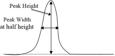
图 2。一个基本示例的曲线峰值高度和宽度,将与其相乘 (峰值高度乘以宽度在 ½ 高度)。
采用高效液相色谱是能够量化的每个基于标准 (图 3) 的校准曲线的所有样本的 3 组件。
从这套实验,它确定这些减肥苏打水 12 盎司可以载支付下列金额,每个组件:
健怡可乐: 50.5 毫克咖啡因;阿斯巴甜 217.6 毫克;83.6 毫克苯甲酸。
零度可乐: 43.1 毫克咖啡因;阿斯巴甜 124.9 毫克;85.3 毫克苯甲酸。
百事轻怡: 34.1 毫克咖啡因;阿斯巴甜 184.7 毫克;79.5 毫克苯甲酸。
不足为奇的是,所有 3 约有同样数量的苯甲酸酯,因为它是只是一种防腐剂。焦炭产品有更多的咖啡因,和零度可乐已经少得多阿斯巴甜比其他两个的苏打水,因为它也包括柠檬酸为一些调味料。
下面的编号是实际大量咖啡因和阿斯巴甜在 12 盎司罐头的 3 种饮食苏打水 (咖啡因含量制得的可口可乐和百事可乐的网站。阿斯巴甜内容被从网上和 DiabetesSelfManagement.com):。
健怡可乐: 46 毫克咖啡因;阿斯巴甜 187.5 毫克
零度可乐: 34 毫克咖啡因;阿斯巴甜 87.0 毫克
百事轻怡: 35 毫克咖啡因;阿斯巴甜 177.0 毫克
计算示例 (表 2):
浓度的咖啡因在 STD #1: 咖啡因的组件解决方案有 0.400 g 的咖啡因稀释至 500 毫升 = 0.500 L → 0.800 g/L = 0.800 毫克/毫升。
STD #1 有 1 毫升的稀释至 50.0 mL 此解决方案
0.800 毫克/毫升 * (1.0 毫升/50.0 mL) = 0.016 毫克/毫升 = 16.0 毫克/升。
STD #2 了 2 毫升的稀释至 50.0 mL 此解决方案
0.800 毫克/毫升 * (2.0 毫升/50.0 mL) = 0.032 毫克/毫升 = 32.0 毫克/升。
从三个校准图 (图 4) 结果产生了以下等式:
咖啡因峰面积 = 0.1583* [咖啡因 mg/L]-0.574
阿斯巴甜峰面积 = 0.02696* [阿斯巴甜 mg/L]-0.405
苯甲酸峰面积 = 0.1363* [苯甲酸 mg/L]-1.192
健怡可乐: 咖啡因峰面积 = 10.68 = 0.1583* [咖啡因 mg/L]-0.574
[咖啡因 mg/L] = (10.68 + 0.574) / (0.1583) = 注入样品中 71.1 毫克/升。
自从 2 倍稀释,健怡可乐了 141.2 mg/L 咖啡因。
每个 12 盎司的金额可以 = (141.2 毫克/升) (0.3549 毫升/12 盎司 can) = 50.5 毫克咖啡因 / 可以。
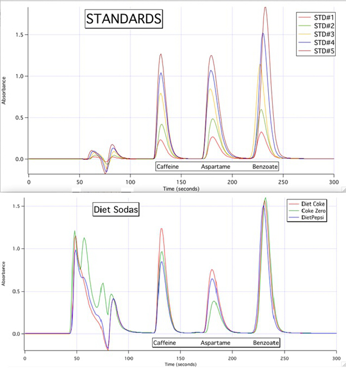
图 3。高效液相色谱-5 标准和 3 个样品。
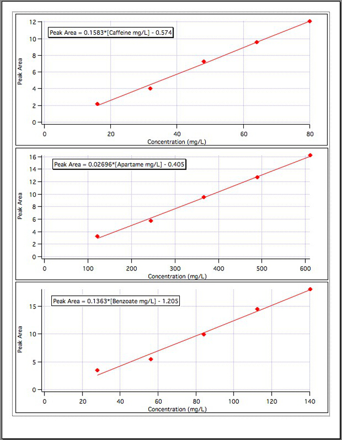
图 4。每个 3 组件校准曲线。
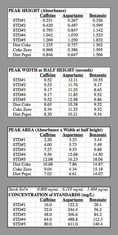
表 2。用于生成校准曲线的高效液相色谱法试验数据表格。
高效液相色谱法是一种广泛用于技术在分离和检测对于许多应用程序。它是理想的非挥发性化合物,作为气相色谱 (GC) 要求,样品都放在他们的气相。非挥发性化合物包括糖、 维生素、 药物,以及代谢物。它也非破坏性的它允许每个组件必须收集为进一步分析 (例如质谱)。流动相是几乎是无限的它允许对极性的 ph 值,以实现更高的分辨率的更改。在实际试验中的梯度流动相使用允许这些变化。
对可能与人工甜味剂阿斯巴甜的可能的健康问题甚表关注。当前产品标签不显示这些组件在饮食饮料的量。此方法允许为量化这些款额及咖啡因和苯甲酸。
其他应用程序包括确定数额的农药在水中;确定所用的对乙酰氨基酚或布洛芬在疼痛缓解片;确定是否有提高成绩的药物存在于血液中的运动员;或简单地确定毒品犯罪实验室中的存在。虽然这些样品的浓度和经常身份的组件,可以很容易确定,一个限制是,几个样本可能会接近相同的保留时间,从而导致共同洗脱。
Tags
ABOUT JoVE
Copyright © 2024 MyJoVE Corporation. All rights reserved