
Measuring Turbulent Flows
Overview
Source: Ricardo Mejia-Alvarez and Hussam Hikmat Jabbar, Department of Mechanical Engineering, Michigan State University, East Lansing, MI
Turbulent flows exhibit very high frequency fluctuations that require instruments with high time-resolution for their appropriate characterization. Hot-wire anemometers have a short enough time-response to fulfill this requirement. The purpose of this experiment is to demonstrate the use of hot-wire anemometry to characterize a turbulent jet.
In this experiment, a previously calibrated hot-wire probe will be used to obtain velocity measurements at different positions within the jet. Finally, we will demonstrate a basic statistical analysis of the data to characterize the turbulent field.
Procedure
- Measure the width of the slit, W, and record this value in table 1.
- Set the hot-wire anemometer at a distance from the exit equal to x = 1.5W along the centerline. Record this streamwise position in table 2. The centerline is the origin of the spanwise coordinate (y = 0).
- Start the data acquisition program for traversing the jet. Set the sample rate at 500 Hz for a total of 5000 samples (i.e. 10s of data).
- Record the current spanwise position of the hot-wire in table 3.
Results
Figure 5 shows the distribution of average velocity across the jet at the downstream position x = 3W. And Figure 6 shows the distribution of turbulence intensity across the jet at the same downstream position. Table 3 has the results for the local values of average velocity and turbulence intensity at the streamwise position x = 3W. The last column of this table is the ratio between the local v
Application and Summary
This experiment demonstrated the application of hot-wire anemometry for characterizing turbulent flows. Given that turbulence exhibits high frequency velocity fluctuations, hot-wire anemometers are suitable instruments for its characterization due to their high time-resolution. With this in mind, we used a calibrated hot-wire anemometer to characterize the average local velocity and turbulence intensity at different positions within a planar jet. These quantities were determined using statistical descriptors for turbulen
References
- Chapra, S.C. and R.P. Canale. Numerical methods for engineers. Vol. 2. New York: McGraw-Hill, 1998.
- King, L.V. On the convection of heat from small cylinders in a stream of fluid: determination of the convection constants of small platinum wires with applications to hot-wire anemometry. Philosophical Transactions of the Royal Society of London. Series A, Containing Papers of a Mathematical or Physical Character 214 (1914): 373-432.
- White, F. M. Fluid Mechanics, 7th ed., McGraw-Hill, 2009.
- Munson, B.R., D.F. Young, T.H. Okiishi. Fundamentals of Fluid Mechanics. 5th ed., Wiley, 2006.
- Buckingham, E. Note on contraction coefficients of jets of gas. Journal of Research,6:765-775, 1931.
 mm).
mm). mm).
mm).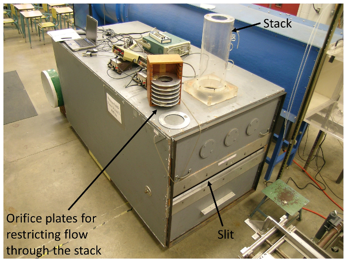
Skip to...
Videos from this collection:

Now Playing
Measuring Turbulent Flows
Mechanical Engineering
13.5K Views

Buoyancy and Drag on Immersed Bodies
Mechanical Engineering
30.0K Views

Stability of Floating Vessels
Mechanical Engineering
22.6K Views

Propulsion and Thrust
Mechanical Engineering
21.7K Views

Piping Networks and Pressure Losses
Mechanical Engineering
58.1K Views

Quenching and Boiling
Mechanical Engineering
7.7K Views

Hydraulic Jumps
Mechanical Engineering
41.0K Views

Heat Exchanger Analysis
Mechanical Engineering
28.0K Views

Introduction to Refrigeration
Mechanical Engineering
24.7K Views

Hot Wire Anemometry
Mechanical Engineering
15.6K Views

Visualization of Flow Past a Bluff Body
Mechanical Engineering
11.9K Views

Jet Impinging on an Inclined Plate
Mechanical Engineering
10.7K Views

Conservation of Energy Approach to System Analysis
Mechanical Engineering
7.4K Views

Mass Conservation and Flow Rate Measurements
Mechanical Engineering
22.6K Views

Determination of Impingement Forces on a Flat Plate with the Control Volume Method
Mechanical Engineering
26.0K Views
Copyright © 2025 MyJoVE Corporation. All rights reserved