RVB et l’imagerie spectrale racine pour le phénotypage de l’usine et la recherche en physiologie : montage expérimental et des protocoles d’imagerie

Résumé

Un protocole expérimental est présenté pour évaluation des sols cultivés des systèmes racinaires plante avec RVB et imagerie hyperspectrale. Combinaison du temps d’image RVB scanne de série avec les informations de Chimiométrie de hyperspectral optimise les aperçus de la dynamique des racines végétales.

Résumé

Meilleure compréhension des dynamiques de racine de plante est indispensable pour améliorer l’utilisation efficace des ressources des systèmes agricoles et augmenter la résistance des cultivars de contre les stress environnementaux. Un protocole expérimental est présenté pour RVB et imagerie hyperspectrale des systèmes racinaires. L’approche utilise rhizoboxes où les plantes poussent dans les sols naturels au cours de plus de temps pour observer des systèmes racinaires entièrement développées. Les paramètres expérimentaux sont illustrées pour évaluer rhizobox des plantes sous stress hydrique et d’étudier le rôle des racines. Une installation d’imagerie RVB est décrite pour la quantification rapide et bon marchée du développement racinaire au fil du temps. Imagerie hyperspectrale améliore la segmentation de la racine de l’arrière-plan du sol par rapport au Seuillage couleur RVB. La force particulière de l’imagerie hyperspectrale est l’acquisition d’informations chimiométriques sur le système de racine-sol pour compréhension fonctionnelle. Cela est démontré avec cartographie contenu eau de haute résolution. Imagerie spectrale est toutefois plus complexe dans l’acquisition d’images, de traitement et d’analyse par rapport à l’approche de RVB. Une combinaison des deux méthodes peut optimiser une évaluation détaillée du système racinaire. Exemples d’applications intégrant les traits au-dessus du sol et racine sont donnés dans le contexte de la recherche en physiologie végétale phénotypage et plante. Amélioration de l’imagerie de la racine peut être obtenue en optimisant la qualité de l’image RVB avec le meilleur éclairage à l’aide de différentes sources de lumière et par extension des méthodes d’analyse image à déduire sur les propriétés de la zone racine de données spectrales.

Introduction

Racines offrent plusieurs fonctions essentielles pour les plantes telles que le stockage des assimilats, ancrage des plantes terrestres dans le sol et l’absorption et le transport de l’eau et les nutriments¹. Du point de vue évolutif, la formation des axes racine est considérée comme une condition préalable fondamentale à l’origine des plantes de terre². Malgré ce rôle important, historiquement les racines ont occupé seulement une position marginale dans la recherche biologique. Plus ces derniers temps, cependant, il est scientifique un intérêt croissant dans des systèmes de racine de plante comme en témoigne la Figure 1.

Figure 1 : Importance des racines plant sciences.
Nombre de racines des études en pourcentage de toutes les études de plantes publiés dans des revues SCI connexes au cours des dernières décennies. Résultat de Scopus en utilisant les mots-clés « plante » et « des plantes et racines » de recherche. S’il vous plaît cliquez ici pour visionner une version agrandie de cette figure.

Deux raisons principales peuvent être hypothétiquement sous-tendent les récentes avancées dans la recherche de la racine. Première végétation terrestre est exposée à des stress environnementaux plus fréquents à la suite de changements mondiaux³. Dans le contexte de la production agricole végétale, on estime que dans le monde environ 30 % de la surface agricole sont limitées par l’eau et phosphore^4,5. Réduction du stress du rendement des cultures sont des raisons principales pour les écarts de rendement importantes qui sont estimés dans le monde au moins 50 % de la productivité potentielle pour les cultures pluviales agro-écosystèmes⁶. En plus de la disponibilité des ressources faibles, cela est également liée à l’efficacité d’utilisation de ressources pauvres, c'est-à-dire insuffisante capacité d’une usine d’exploiter les ressources disponibles⁷. Cela se traduit par des pertes de ressources mobiles tels que le nitrate qui peut affecter négativement les autres écosystèmes. L’efficacité d’utilisation globale d’azote actuel par exemple est estimée à 47 %⁸. Meilleure ressource efficience grâce à des méthodes de gestion améliorée de l’utilisation et des cultivars est donc d’une grande importance pour les deux une croissance de la production agricole aussi bien en ce qui concerne la durabilité de l’environnement. Dans cette usine de contexte racines sont considérés comme un objectif clé pour l’amélioration des cultures et culture systèmes^9,10.

Un deuxième fond important pour l’intérêt récent pour les racines des plantes est une avancée technologique dans les méthodes de mesure. Méthodes de racine ont longtemps été limités par deux grands défis : pour la mesure des racines de plantes qui poussent dans le sol, ils devaient être isolés pour la quantification, pour la plupart en lavant¹¹, ainsi déranger la disposition architecturale des axes de racine. Observation de racine in situ à l’aide d’excavation méthodes, conservant ainsi la situation naturelle des racines dans le sol, ont été utilisés pour la description botanique¹². Encore, ils sont très coûteuses en temps et donc ne répondent pas aux exigences de débit d’analyse comparative système structural-fonctionnelle de la racine. D’autre part haut débit des méthodes pour la mesure d’architecture de racine ont été faites principalement sur des milieux artificiels et pour des semis de plantes¹³ où l’extrapolation à l’environnement naturel de croissance des plantes est discutable¹⁴.

Le boom récent de recherche de la racine est intimement lié à l’avance en imagerie méthodes¹⁵. Imagerie des approches en études de racine peut être grossièrement regroupé en trois types. Tout d’abord il y a des méthodes 3D haute résolution tels que CT et IRM¹⁶. Ces méthodes sont plus aptes à étudier les processus d’interaction des racines avec le sol, tels que la sécheresse provoquée par le xylème embolie¹⁷. En général, ils sont appliqués aux échantillons relativement petits où ils permettent des observations détaillées. Une comparaison de CT et MRI pour pots de tailles différente et l’imagerie de radicelles est fournie en¹⁸. Deuxièmement, il y a de^19,des méthodes d’imagerie haut débit²⁰. Ces méthodes sont pour la plupart sur la base commune 2D RGB imagerie des racines qui poussent sur des milieux artificiels (gel, papier de germination) où contraste élevé permettant une dissection relativement simple entre racines et l’arrière-plan. Elles sont appropriées pour la comparaison à haut débit entre traits racine des plantules de génotypes de cultures différentes en vertu de conditions artificielles normalisés croissant¹³. Entre ces deux approches sont rhizobox méthodes : ils utilisent l’imagerie 2D des racines qui poussent dans le sol sur longue période et ont un débit moyen de^21,22. Un défi récent à l’imagerie de la racine (2D) consiste à capturer également indicateurs de fonctionnalité de racine en plus de la description de la structure²³.

Dans le présent document, nous présentons les protocoles expérimentaux d’imagerie rhizobox cultivé le système racinaire à l’aide de (i) une simple et peu coûteuse sur mesure RVB d’imagerie configuration et (ii) une installation d’imagerie de NIR plus complexe. Exemple résultats obtenus de ces deux configurations sont montrés et discutés dans le contexte de phénotypage de plante et de la recherche en physiologie végétale.

Protocole

1. Rhizoboxes for plant growth

NOTE: The experimental system uses rhizoboxes to grow plants for root imaging. First the design of the boxes and the substrate used are described, and then details on the filling procedure are given.

1. Design of rhizoboxes
   1. Create rhizoboxes (Figure 2) with a back plate and side frames made of grey PVC with 15 mm strength. Use a box size of 300 mm x 1000 mm. For the front window, use 6 mm mineral glass which is attached to the PVC frame by metal rails being screwed into the side walls.
   2. Create three holes on the bottom frame to allow drainage of excess water. These holes can be optionally closed by plastic screws.
   3. Before filling, adapt the inner diameter of the rhizobox (between 10 mm and 30 mm) by inserting PC multiwall sheets. An inner space of 10 mm is recommended for most crops to reduce the weight (rhizobox weight without soil is 13.2 kg) of the entire system.

Figure 2: Rhizobox experimental system and its components.
Left figure shows the dimensions of a rhizobox and right figure its single components, being a grey PVC back plate with side frame, a front mineral glass, multiwall sheets for variable inner diameter and metal angles to fix the front glass to the back compartment. Please click here to view a larger version of this figure.

2. Substrate
   1. Fill the rhizoboxes with field soil (for this experiment: silt loam top soil from a calcareous chernozem) sieved to 2 mm particle size.
   2. Open the rhizoboxes for filling the substrate into the inner compartment (back plate with side frames) in horizontal position using pre-wetted substrate. Fill horizontally to avoid layering and segregation between fine and coarse particles which occurs when filling in vertical position by pouring the substrate through the upper opening.
   3. Pre-wet the substrate before filling. Depending on the type of substrate (particularly on its silt and clay content), do not exceed a water content of 0.12-0.18 cm³*cm^-3 to avoid smearing and structure degradation. Add the difference between pre-mixing and target water content after filling the substrate into the rhizoboxes.
      NOTE: Filling with (oven-)dry substrate and subsequent addition of the entire water is not recommended as is can result in strong settlement of the substrate and formation of large cracks.
3. Step by step filling example
   1. Define the target water content. Here it is initially set at 80% plant available water (PAW) where plants do not suffer from any water shortage.
   2. Determine field capacity (FC) and permanent wilting point (PWP) of the substrate. Here obtain FC using a PVC tube of equivalent height (100 cm) as the rhizoboxes.
      1. Close the tube at the bottom with a stubble having small drainage holes, add 1 cm of gravel to avoid closure of the holes from finer substrate and fill the substrate to the same bulk density as used for the rhizoboxes (1.3 g cm^-3).
      2. Saturate the tube with water until drainage occurs and leave it for two days to equilibrate (the resulting water content is per definition equivalent to field capacity), while covering the upper opening with cling-film to avoid evaporation. The field capacity value achieved for the soil in this experiment was 0.357 cm³ cm^-3.
         NOTE: Water content at PWP has to be known in advance from standard soil physical methods (e.g. pressure plate measurements²⁴) or from texture based pedotranfer functions²⁵. Here it is equal 0.12 cm³ cm^-3 for the soil used.
      3. When measuring FC by pressure plate extraction too, take the water content at a matrix potential of h=-100 hPa and not h=-330 hPa in order to correspond to the rhizobox geometry (height of 100 cm = 100 hPa).
      4. Calculate the water content (WC) at 80% PAW: WC (cm³ cm^-3) = 0.80 (FC-PWP) + PWP. For the hydraulic limits of the soil used here this gives a volumetric water content at 80% PAW of 0.31 cm³ cm^-3.
      5. Calculate the water amount for a rhizobox volume of 2850 cm³ (30 cm width, 1 cm inner space, 95 cm in height, with top 5 cm keeping free of substrate for watering). This gives a water volume of 883.5 cm³ equal 883.5 g for the density of water being 1.0 g cm^-3 at 20 °C.
   3. Define the bulk density (d_b) to fill the rhizoboxes. Here, set at 1.3 g cm^-3 corresponding to values typically found in agricultural field soils. The amount of dry substrate required to fill a rhizobox volume of 2850 cm³ at this d_b equals 3705 g of dry soil.
   4. Pre-wet the dry soil to a gravimetric water content of 0.108 g g^-1 (equal to a volumetric water content of 0.14 cm³ cm^-3) by adding 400 g of water for 3705 g of dry soil and mix it gently to obtain a homogeneous water distribution. Manually disrupt larger aggregates to keep the particle size ≤ 2 mm.
   5. Fill the pre-wetted soil into the opened rhizoboxes and compact it gently using a polystyrene sheet (30 x 10 x 1.5 cm) to cover the inner volume of the box, thereby resulting in a homogeneous d_b of 1.3 g cm^-3.
   6. Add the remaining amount of water (483.2 g) to achieve the target water content of 0.31 cm³ cm^-3 by spraying onto the surface with a spray bottle. Ensure small drop size to avoid surface structure degradation and homogeneous wetting. Keep the box on a balance during spraying to monitor the amount of water actually added to substrate.
   7. Let the water redistribute for 10 minutes and then press the glass onto the surface and fix it with the side metal rails. The average final weight of rhizoboxes with wetted substrate was 17818 ± 68 g (13230 g rhizobox weight + 3705 g dry soil + 883 g water).
      NOTE: The homogeneous water content filled in the horizontal boxes will redistribute when the boxes are set in their final position according to the resulting potential gradient. This is a physical process in all plant growth pots according to their geometry (height) and experimenters should be conscious on their pot hydraulics²⁶.

2. Climate room setup

1. Equip the climate room (Figure 3) with 8 LED lamps providing homogeneous illumination of 450 μmol m^-2 s^-1 with spectral peaks at 440 (blue) and 660 (red) nm for optimum plant growth.

Figure 3: Climate chamber with rhizoboxes for stress experiment.
(A) Left view of entire chamber with LED illumination, weather station and PC (here for logging leaf hygrometers); right view with a close-up of the metal frame holding rhizoboxes in 45 ° inclination and wooden plates used to shied rhizobox glass window against light. (B) Stress experiment with sugar beet combining four stages with stress due to different atmospheric demand (high/low) and soil water availability (high/low). Green bars of mean stomata conductance give an indication of plant stress response. Please click here to view a larger version of this figure.

2. Set the ambient parameters according to plant/experimental needs. Here, use 14 hours light and 10 hours dark for illumination. During plant establishment and before stress treatments started, set the temperature to 20° C during day and 15° C during night and keep relative humidity at 50 ± 8%.
3. Put the rhizoboxes at an inclination of 45° using an adequate metal framework. This maximizes root growth towards the glass surface due to gravitropism.
4. Cover the glass window by a wooden plate to keep the root zone in dark and avoid algae growth due to light penetrating through the glass surface.

3. Sugar beet example setup and treatments

1. Pre-germinate sugar beet seeds on wet filter paper for three days at 20 °C in an incubator until the radicle emerges. This ensures seeding with viable plants.
   NOTE: Pre-germination is not required for plants with high germination vigor, thereby avoiding the risk of damaging the radicle at seeding. For sugar beet seeds with a thick pericarp, however the risk of non-viable seeds is high and pre-germination significantly accelerates the emergence of the radicle compared to direct seeding into soil.
2. Drill a small hole to about 1.5 cm soil depth in the middle of the rhizobox with a screwdriver, position one seed in it using tweezers with the radicle oriented downwards and next to the glass window (this improves the initial visibility) and gently cover it with soil.
3. Add a 0.5 cm layer of fine gravel (2-4 mm) on top of soil to protect the soil aggregates from slaking during irrigation and reduce evaporation losses. To facilitate emergence, keep the soil surface free of gravel where the seed has been positioned.
4. Add 10 g of water to enhance establishment.
5. During establishment and early growth until experimental stress treatments start, irrigate the rhizoboxes every 2-4 days to keep the initial moisture content of 80% PAW.
   1. Determine the amount of irrigation water required by weighing the rhizoboxes and adding water until achieving the initial weight of each individual box. For manual irrigation use a pipette to avoid surface structure degradation during watering.
6. Arrange the rhizoboxes according to the established design in the climate room. The protocol reported here is based on an experiment with six sugar beet cultivars in five replicates in a completely randomized design (CRD).
   1. Reposition rhizoboxes each time when taking them out of the metal holder for weighing and watering. This avoids any effects of residual (light) inhomogeneity inside the climate room.
7. Define the time for onset of stress treatments and the type of stress. The following settings (Figure 4) are used here.
   1. Start measurements at BBCH 15 (five leaves unfolded) with roots covering around 75% of the rhizobox depth and the canopy being sufficiently developed for measurements at the leaves. Keep each stage for at least three days to ensure adaptation to the new settings and make measurement.
   2. For the non-stress observations keep the initial settings with optimum soil moisture (80% PAW) and ambient conditions (20° C/15° C temperature, 50 ± 8% rH) giving a daytime vapor pressure deficit (VPD) of 1.28 ± 0.1 kPa (cf. Figure 3 C).
   3. Raise the atmospheric demand to a daytime VPD of 2.45 ± 0.4 kPa by increasing the temperature to 27°C/20°C and decreasing rH to 35%, while keeping soil moisture at 80% PAW.
   4. Subsequently dry down the rhizoboxes to 40% PAW equivalent to a water content of 0.215 cm³ cm^-3 by withholding irrigation. Reset the initial ambient conditions with low atmospheric demand (VPD of 1.28 kPa).
   5. Combine stresses increasing the atmospheric demand to a VPD of 2.45 kPa and keep soil moisture at 40% PAW.

4. Root imaging methods

1. Combine imaging methods to make use of their respective advantages and depending on the information targeted.
   1. Apply RGB imaging in the VIS range to track root growth, architecture and morphology over time which implicitly requires frequent measurement. Advantages of RGB imaging are (i) low costs, (ii) rapid image acquisition, (iii) low requirements of hard-disk space (image size: 48 MB) and (iv) high resolution (3648 x 5472 pixels).
   2. Use hyperspectral imaging (HSI) in the NIR range when chemometric features of root and soil are required. Advantages are (i) spectral features for segmentation between roots and soil background and (ii) access to physico-chemical system properties (e.g. soil water content, root age). Disadvantages are (i) higher scanning time (about 16 minutes per rhizobox), (ii) large size of datasets (13.7 GB per rhizobox image) and (iii) lower resolution of the NIR camera (320 x 256 Pixel), and (iv) higher complexity of data analysis.
2. RGB root imaging
   1. Use an imaging box (Figure 4) that shields from ambient light and fixes the camera position consisting of a metal frame with a width of 1 m and a height of 1 m with side walls lined with pressboards. At the front end, fix the camera at two positions at a distance of 80 cm from the rhizobox.
      1. Attach a tapeline on the rhizobox frame with transparent adhesive tape and position the rhizobox in the holder of the imaging box.
      2. Illuminate the rhizobox using four 24 W fluorescent light tubes attached at a distance of 80 cm from the rhizobox. Also, mount four 15 W UV tubes at 20 cm from the rhizobox as alternative illumination making use of root auto-fluorescence in case of low contrast between root and (bright colored) substrate background.
      3. Take two images (top and bottom position) to cover the upper and the lower half of a rhizobox with an overlap of about 3 cm.
   2. Acquire RGB images with a digital single-lens reflex camera which is fixed by quick release plates on the respective positions of the imaging box.
      1. Apply the following settings when using the fluorescent light tubes. Adapt these example settings for any changes in dimensions and illumination as well as the camera model.
         1. Turn off autofocus and stabilizer on the camera objective. Set camera to manual mode.
         2. Set ISO speed to 500. Set shutter speed to 13. Set Aperture to 5.6.
         3. Turn off the mirror lock. Set the white balance to Auto White Balance.
      2. Use the following settings for illumination with UV tubes:
         1. Turn off autofocus and stabilizer on the camera objective. Set camera in manual mode.
         2. Set ISO speed to 1000. Set shutter speed to 13. Set Aperture to 5.6.
         3. Turn off the mirror lock. Set the white balance to Fluorescence.
   3. Merge the RGB images from top and bottom of the rhizobox into a single image a photo editor (e.g., Adobe Photoshop). Use the tapeline at the side frame of the rhizoboxes and control overlapping objects (root and soil features).
      1. Copy the two separate images, each with pixels size of 3648 x 5472, into a new file of size 3648 x 10944 pixels and white background.
      2. Reduce the layer opacity for one image to 60% and align overlapping parts of the images (tapeline, objects). Thereafter restore layer opacity to 100%.
      3. Based on the ruler on the image add two red lines of exactly 1 cm to the top of the image where no roots are present. These lines are later used at image analysis to scale the image to correct length dimensions.
      4. Merge all layers and remove parts of the image outside the soil filled window with the cropping tool.
      5. Save the image as tiff-file for further analysis.
      6. In case of images with UV illumination, reduce colors to greyscale before saving using the toolbar Adjustments-Black & White, and selecting the predefined High Contrast Blue filter.
   4. For segmentation between roots and soil background as well as for quantification of root traits of interest (e.g. length, surface, diameter, branching) use any root analysis software (see www.plant-image-analysis.org for available tools). Here WinRhizo is used.
      1. Open the rhizobox tiff-image the software.
      2. Calibrate the length scale of the image using the scaling bars added to the image.
      3. Select Based on Color in the Analysis menu where selecting Root & Background Distinction.
      4. Define a calibration file with color classes corresponding to roots and soil (background). For the example images used here (cf. Figure 8) three root color classes (old laterals, young laterals, tap root) and three soil color classes are defined.
      5. For the greyscale images (UV-illumination) select (i) Based on grey levels, and (ii) Pale Root on Black Background in the Root & Background Distinction menu and use a local Lagarde intensity threshold for segmentation.
      6. Open a data file where results are saved.
      7. Run the analysis and subsequently control whether there are regions (e.g. at the edges) which are mismatched. In this case define an exclusion region and restart the analysis. For roots not classified, add additional color classes and restart the analysis. For elements wrongly classified as roots, activate/increase the Debris & Rough Edges filtering options.

Figure 4: Imaging box to acquire RGB rhizoboxes pictures.
Left view of front side where rhizoboxes are attached for imaging with light sources inside; right view of backside where the camera is mounted. Please click here to view a larger version of this figure.

3. Hyperspectral root imaging
   1. Hardware setup
      1. Use a hyperspectral root imaging system (Figure 5) consisting of (i) a thermo-electrically cooled 14-bit monochrome NIR camera with a spectral range from 900 nm to 1700 nm, 320 by 256 pixels and a frame rate of 100Hz and (ii) an imaging spectrograph with a spectral range 900 nm to 2500 nm and a spectral resolution of 3.6 nm. Arrange a halogen line illumination source (four 50 W halogen spots) in a 45°/-45° geometry. Mount the imaging sensor on a two-axis positioning system. The scan window has a size of 240 x 1000 mm, i.e. 30 mm at each edge of the rhizobox are not covered by the image.
      2. Control the system by a Matlab script for (i) white and dark standard acquisition, (ii) setting of camera integration time, (iii) selecting spatial (pixel size 0.1 mm; pixel size 1.0 mm) and spectral resolution (all 222 spectral bands with a resolution of 3.6 nm; smoothed spectrum with 54 bands and a resolution of 14.8 nm), and (iv) defining the scan region on the rhizobox.
      3. Save images as SIF-files. To avoid problems during saving of large files, subdivide each scanned image stride (9 strides per rhizobox) into four segments (three of 300 mm length, one of 100 mm length) and save separately with a unique file name consisting of stride number (1 to 9) and part (1 to 4) as well as date and time (YYYY.MM.DD HH:MM:SS). An entire rhizobox scan requires a hard-disk space of 13.7 GB.
   2. Image acquisition and analysis.
      NOTE: Figure 6 shows the steps of image acquisition, segmentation and analysis.
      1. Image acquisition comprises selection of camera setting for optimum image quality and definition of scan parameters.
         1. Determine the camera integration times for the rhizobox scan and the white standard in the camera software.
            1. Open the imaging GUI and move the camera to a position of the rhizobox where roots are present.
            2. Adjust the integration time of the camera targeting a light object (i.e. root) in a way that approximately 85% of the full dynamic range of the camera is used on the histogram displayed by the software. Repeat for the white standard by moving the camera positioning system to target the white standard. Then close the camera software.
         2. Open the Matlab Imaging GUI and make all settings for the current rhizobox scan. For the data reported here, use the following settings:
            Integration time white standard: 1000
            Integration time rhizobox: 4000
            Spectral resolution: Full resolution (i.e. 222 narrow-range spectral bands)
            Full spatial resolution (pixel size of 0.1 mm)
            1. Acquire the dark and white standards before each imaging run, e.g. once a day. The dark standard represents the camera noise, while the white standard gives the maximum reflectivity. These data are required for image normalization during pre-processing.
            2. Define whether the entire rhizobox or only part of it is scanned. For the present case entire rhizoboxes are imaged. Then start the scan.
      2. Process the image with a Matlab script. Operations performed by the script are described.
         NOTE: Scripts are currently in an undocumented version and can be obtained from the corresponding author. After proper documentation, they will be available for download from the website of the corresponding author's institution (www.dnw.boku.ac.at/pb/).
         1. Compose an entire image stride from the rhizobox center (containing roots) merging the four parts of the stride.
            NOTE: At this stage it is neither necessary nor recommended to use a spectral image of an entire rhizobox (i.e. all 9 strides) as the file size will make each calculation step in Matlab very time consuming and the information contained in one central stride is sufficient for the first steps of image analysis.
         2. Normalize the image using the acquired dark and white standards and taking into account the different integration times of white standard and rhizobox scans which are saved automatically during scanning in a file.
         3. Optionally apply a smoothing filter to remove noise from the image. The script currently offers 3x3 kernel median filtering and multiple scatter correction. For the image evaluation presented here, no filters are applied.
         4. Display the image at all recorded spectral bands to obtain a first insight and decide a wavelength to be displaying for selecting regions of interest (cf. image segmentation).
      3. Perform segmentation between roots and soil background in a separate script with the following steps.
         1. Select regions of interest (ROI) for root and soil to find spectral features for segmentation. Use the freehand selection tool to mark a ROI on the image displayed at a wavelength previously identified with good contrast between roots and soil. Here, use three ROIs on the root (old and young laterals, tap root) and two ROIs in the soil (dry, wet region).
         2. Display a rectangle with the selected ROIs and the remaining part as a black mask and visualize the selected ROI image at all wavelengths.
         3. Remove all lines in the image matrix containing pixels of spectral intensity = 0 (black pixels).
         4. Fuse the root and soil ROIs into one foreground (root) and one background (soil) matrix for segmentation.
         5. Search spectral bands (intensity of single spectra or spectral ratios) providing the best separation between root foreground and soil background²⁷. Quantify the distinction between the resulting pixel histograms for root and soil using Bhattacharyya distance²⁸.
         6. Select a threshold intensity value separating the histograms.
         7. Create a binary image by applying the selected threshold to the original image. This sets all pixels having smaller intensity than the threshold to zero and those with higher intensity to one (done automatically be the script).
         8. Save the binary image as tiff-file.
      4. Open the binary image and analyze root traits. Select (i) Based on grey levels, and (ii) Pale Root on Black Background in the Root & Background Distinction menu and use global intensity threshold (the image is already binarized).
      5. For mapping the water content from the hyperspectral data acquire a calibration dataset and apply a calibration equation to a rhizobox image.
         1. Subdivide a rhizobox into 5 cm compartments using polystyrene sheets to fill them with soil (same substrate and d_b as used for the experiment) at different water contents (Figure 8).
         2. Calculate the respective amounts of water to be mixed with soil and fill the compartments (same procedure as described in 1.3. for the entire rhizobox).
         3. Scan the calibration rhizobox with the same settings as used for the planted rhizoboxes.
         4. Perform the following steps using a script.
            1. Merge the four parts of a stride from the water calibration box to one stride and normalize it with dark and white standards.
            2. Select rectangular boxes at each compartment with different water content and save them in a structure array.
            3. Determine the spectral feature that best separates the water content compartments. This is done with a search algorithm for the global maximum of the intensity differences between mean spectra of adjacent water contents.
            4. Calculate the mean spectral intensity value for this feature for each water content compartment of the calibration rhizobox.
            5. Fit a regression equation through the directly measured water content and the respective spectral quantifier.
            6. Apply the regression equation to each pixel not classified as root on a rhizobox image and for the spectral feature (band) determined above which best relates to water content.

Figure 5: Hyperspectral root scanner.
The main components of the scanner are indicated. The small picture shows the camera during imaging of a rhizobox. Please click here to view a larger version of this figure.

Figure 6: Steps in hyperspectral root imaging.
Hyperspectral root imaging consists of three mains steps being (i) image acquisition, (ii) image segmentation and (iii) analysis of the spectral data. Please click here to view a larger version of this figure.

Figure 7: Rhizobox for water calibration.
The rhizobox contains compartments with substrate at different water content which are subdivided by polystyrene sheets. Germination paper at the dry compartments ensures that soil particles do not rinse into neighboring compartments. Please click here to view a larger version of this figure.

5. Application examples

NOTE: Quantitative root information is applied in the context of plant phenotyping (cultivar comparison) and for plant physiological research. The following aboveground data are reported to exemplify these cases.

1. Leaf area: Measure leaf area non-destructively at selected stages during the experiment via the length and width of leaves as a proxy. Alternatively canopy images can be used²⁹.
   1. At the end of the experiment measure leaf length and width together with area of clipped leaves using a leaf area meter. Calibrate the non-destructive method applying a regression equation to the data pairs.
2. Dry matter: At the end of the experiment, measure aboveground dry matter by clipping the plants with scissors and dry them for 24 hours at 105 °C in an oven.
3. Stomata conductance: Measure stomata conductance with a leaf porometer. Before measurement, keep the device for at least one hour in the climate chamber to allow sensors equilibrate with ambient conditions and calibrated the device each time when ambient settings in the climate chamber are changed. Take measurements from at least three leaves per plant.

Résultats

Example results are presented for root segmentation based on RGB and HS imaging. For spectral imaging an example of high resolution water mapping is provided. Finally results are shown that demonstrate the scientific context where image based root data are applied.

RGB based root measurement

Figure 8 shows an RGB root image time series of sugar beet cultivar Ferrara. The images reveal some artefacts from inhomogeneous illumination of the rhizoboxes, with brighter areas along the left side and different brightness at the overlapping area between top and bottom images.

Figure 8: Root growth time series from the RGB imaging.
Pictures show the sugar beet cultivar Ferrara at different days after sowing (DAS). The images show some artefacts due to non-homogeneous illumination at the left side of the image and between top and bottom images. Scale bars, 2 cm. Please click here to view a larger version of this figure.

Figure 9 provides details on root segmentation based on color thresholding for cultivar Ferrara at day after sowing (DAS) 35. As a reference (Figure 9A), a binary image is used where all roots were manually tracked with a Graphic Tablet. The time required for manual tracking of the entire, fully developed, dense sugar beet root system was around four hours. Figure 9B gives a detailed view on a selected area at the top of the image where old lateral roots are present. Here several root axes are not classified by the color threshold. At the bottom (Figure 9C) on the contrary, where white young roots are predominant, the color based segmentation properly classifies all root axes. The binarized root system (Figure 9D) shows a black area at the left side from the illumination artefact which was defined as exclusion region before running quantitative analysis. Figure 9E shows the corresponding pixel histograms of selected features (roots vs. soil) for the red channel of the RGB image from Ferrara at DAS 35. The root pixels (blue color) clearly show three peaks corresponding to bright young laterals, dark old laterals and tap root. The overlap between the old laterals and the soil background is very strong, leading to unclassified root axes (cf. Figure 9B).

Figure 9: Root segmentation using a color threshold.
(A) Manually segmented root system using a Graphic Tablet, (B) area with poorly segmented old root axes in the top and (C) properly segmented young axes in the bottom of the image, and (D) binary image obtained from color based thresholding. (E) Pixel histograms for selected features of the RGB image. Roots are represented by the blue bars with different root types indicated; soil is represented by the red bars. Scale bars in A and D, 2 cm; scale bars in B and C, 1 cm. Please click here to view a larger version of this figure.

The resulting total visible root length quantified for the manually segmented reference image is 1534.1 cm, while the automatized, color based segmentation gives a total root length of 1427.6 cm.

Greyscale images from UV-illumination do not provide an advantage in the case shown here and performed worse compared to color thresholding (root length: 1679.7 cm). Old roots could not be segmented, and there was more noise in the image, probably due to lower light intensity of the UV lamps. However, in case of young roots with high auto-fluorescence and a bright background substrate, UV-illumination can still be an option as shown by an image obtained from another experiment where sand was used as background substrate (Figure 10).

Figure 10: UV illumination to visualize roots on bright background.
Example from a durum wheat root system growing in a rhizobox filled with quartz sand. The rhizobox is imaged with illumination for (A) UV light and (B) fluorescent (day) light. Scale bars, 2 cm. Please click here to view a larger version of this figure.

HSI based root measurements

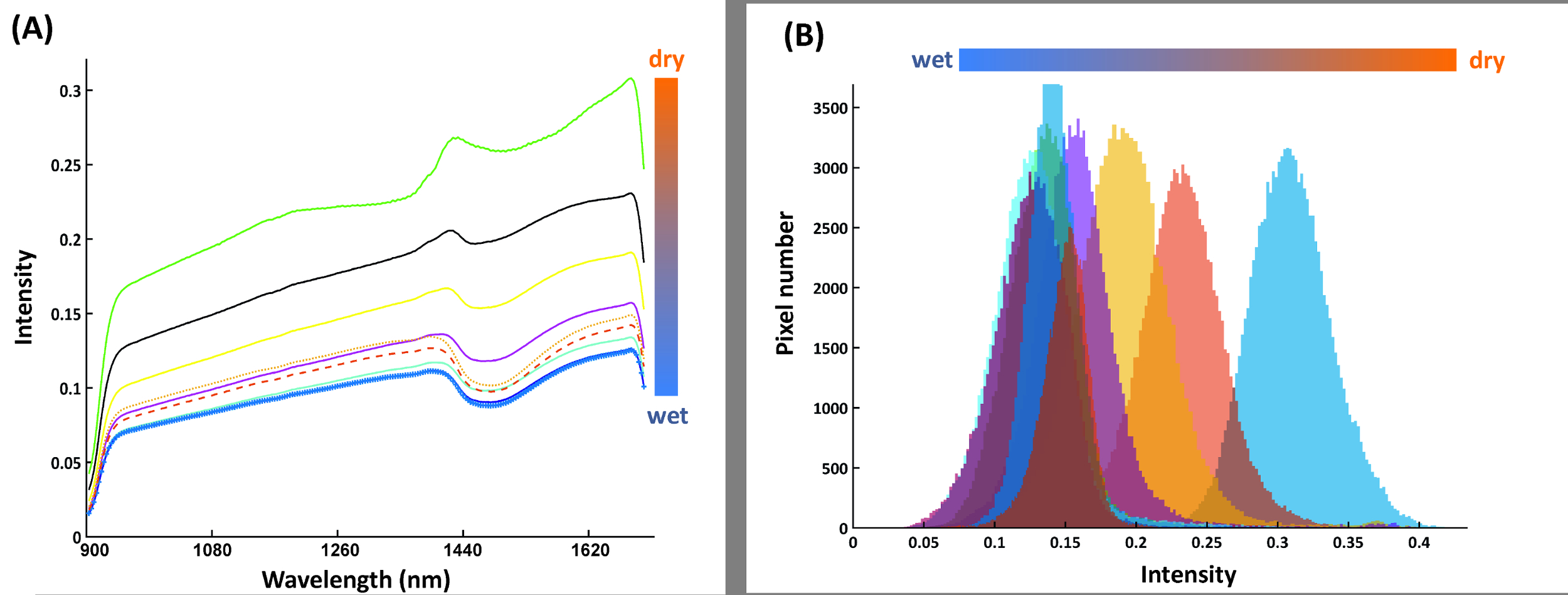
Figure 11 provides the mean spectra for three root ROIs (old and young lateral, tap root) and two soil ROIs (top and bottom of rhizobox).

Figure 11: Mean spectra of root and soil.
Spectra from regions of interest (ROIs) on the root (three root types) and in the soil (top and bottom of the rhizobox). The ROIs are selected to determine an optimum segmentation criterion between root and soil. Please click here to view a larger version of this figure.

It is evident that the tap and young lateral roots differ substantially from the background in intensity of most spectral bands. For the old laterals the intensity differences are much lower. A feature that can be inferred visually is the different slope of the spectrum around water absorption region (1450 nm). Here the slope of root spectra is higher compared to soil spectra. Furthermore a change of tap and young lateral spectra in the region around 1100 nm can be identified that does not occur in the old laterals.

Figure 12A shows the result from the search algorithm identifying a spectral ratio with strongest foreground-background contrast. The ratio of spectra at 1476 nm to 1076 nm provides the best separation between roots and soil. The resulting histogram of root foreground and soil background pixels is shown in Figure 12B. Although there is some overlap, most pixels are clearly separated from the soil background. Fitting a bimodal Gaussian curve through the histogram and using Bhattacharyya distance for quantification, a value of 7.80 is obtained. A value higher 3.0 indicates strong image contrast allowing reliable separation²⁸.

Figure 12: Difference in reflectance between root foreground and soil background for different spectral band ratios and pixel histogram at spectral ratio used for segmentation.
(A) Bright colors (yellow) show high contrast between foreground and background, dark colors (blue) show low contrast. The first 15 bands have been removed because of noise. The red lines indicate the band ratio with highest contrast. (B) Pixel histogram of roots (blue) and soil (red) at segmentation spectral ratio. Blue bars represent the root and red bars the soil. The intensity value corresponds to the ratio of spectral band 160 to spectral band 49. Please click here to view a larger version of this figure.

The binary image (Figure 13) is created by applying a global intensity threshold of the identified spectral ratio at a value of 1.008 calculated from the histogram distance²⁷. Analysis of root length of this image gives a total length of 1557.3 cm which represents an error of only 1.5% compared to the manually tracked reference image.

Figure 13: Binary image of the root system of sugar beet cultivar Ferrara.
The image is obtained by applying a global spectral threshold. Scale bar (bottom left corner), 2 cm. Please click here to view a larger version of this figure.

Although root segmentation has improved using spectral information compared to color based information, the main intention of HS imaging is analysis of chemometric image properties. This is exemplified via mapping the water content of a rhizobox image.

Figure 14A shows the mean spectra of the compartments in the calibration rhizobox (cf. Figure 7) filled with soil of different water content. The shape of spectra is similar between the compartments, i.e. here a spectral ratio does not necessarily provide a more stable classification criterion. Thus intensity at a single spectral band (1680 nm), where the average difference between adjacent water contents is maximized, is identified as best separating criterion. The resulting pixel histograms for this spectral wavelength are shown in Figure 14B.

Figure 14: Spectral features for water content calibration.
(A) Mean spectra of nine water compartments from the calibration rhizobox with different water contents; (B) Pixel histograms for the water compartments at band 216 where average distance between neighboring compartment is maximum. Please click here to view a larger version of this figure.

The relation of the average pixel intensity at 1680 nm and the measured water content is shown in Figure 15.

Figure 15: Relation of spectral reflectance and volumetric water content.
The figure shows data pairs of measured water content and spectral reflectance with empirical curves (linear and exponential) fit to the data excluding the highest water contents (red triangles). Please click here to view a larger version of this figure.

Differentiation of higher water contents from spectral intensity becomes difficult. A significant regression (either linear or exponential) with high R² can be fit to water contents up to around 0.30 cm³ cm^-3. Wetter soil conditions cannot be reliably predicted by the intensity value. Similar behavior of an exponential relation between reflectivity and water content with a decreasing response to water contents higher 0.30 cm³ cm^-3 was also found in other studies³⁰.

A rhizobox image with fine mapping of water content is shown in Figure 16. Four aspects have to be remarked. First, a region of lower water content can be seen in the rooted parts of the rhizobox. Second, strongest depletion is concentrated in the vicinity to single root axes. Third, depletion zones also occur where no root axes are visible on the surface, indicating regions where roots are hidden in soil. Fourth, water mapping without further image-processing results in a patchy appearance due to the aggregated soil. This can indicate inhomogeneous water content distribution at the aggregate scale, but also surface morphology effect on image quality. Chemometric image-processing techniques are an option to overcome such morphological effects in spectral images³¹, but are not implemented so far in the Matlab scripts used here.

Figure 16: Water content mapping on a rhizobox.
The dark blue colours represent regions of high water content, green to red areas show regions with low water content. The plant root is overlaid on the image in black. Scale bar (bottom left corner), 2 cm. Please click here to view a larger version of this figure.

Application examples

Figure 17 relates quantitative root traits from image analysis with aboveground measurements.

Figure 17: Typical application examples for root data.
(A) and (B) show root information used for aboveground-belowground plant characterization in a phenotyping context. (A) represents root growth from the sugar beet cultivar Ferrara, (B) compares six rhizobox grown sugar beet cultivars using leaf-to-root area ratio (data from one replicate). (C) and (D) are functional relations between traits as found in plant physiological research. (C) shows the influence of leaf-to-root area ratio on dry matter production and (D) the relation of root surface area to stomata conductance. Please click here to view a larger version of this figure.

Figure 17A and 17B are relevant for phenotyping focusing on comprehensive aboveground and belowground plant characterization. Figure 17A shows root growth of sugar beet cultivar Ferrara (cf. Figure 8 for images). Expansion of the root system indicates the capacity of a cultivar to explore the soil volume in a given time span of the vegetation period. Figure 17B shows leaf-to-root surface area ratio of six sugar beet cultivars, providing a descriptor for the balance between plant supply (root) and demand (leaf).

Figures 17C and 17D give examples for functional relations of interest in physiological research. In Figure 17C leaf-to-root surface area ratio is related to dry matter formed during the experiment, indicating the predominant role of the assimilating surface as a limiting factor for dry matter accumulation. The lack of significance in spite of a comparatively high R² is related to the low number of paired data (n=6) used here. Figure 17D reveals that cultivars with higher root surface area (improved uptake) have an average higher stomata conductance over the course of the experiment. The higher root area apparently sustains water extraction, thereby prolonging stomata opening.

Discussion

Les protocoles prévoient deux approches complémentaires des sols cultivés imagerie du système racinaire. Une étape cruciale pour des résultats expérimentaux fiables se remplit de la rhizoboxes qui doit s’assurer d’une couche de substrat homogène et même à la vitre avant d’offrir un contact serré racine-sol à la fenêtre d’observation et éviter les trous d’air. C’est la principale raison d’utiliser la terre tamisée relativement fine de < 2 mm : agrégats plus gros aboutir à la morphologie de surface supérieure à la fenêtre d’observation avec des vides entre les agrégats. Outre un risque plus élevé de déshydratation de bout de racine, cela exige également des techniques de traitement des images plus complexes pour la cartographie de l’eau³¹.

Modifications du protocole est donc surtout au remplissage rapide et amélioré de rhizoboxes. Actuellement les temps de remplissage est environ 30 minutes par zone. En outre, utilisation de rhizoboxes avec deux fenêtres en verre pour l’imagerie des deux côtés et modifications pour optimiser l’homogénéité d’éclairage pour les meilleures images RVB sont testés. Prolongation de matériel peut-être aussi envisager d’intégration des optodes planaire³² mais aussi capacité d’imagerie³³ dans le système de rhizobox. Cependant, c’est au-delà des activités actuelles de mise à niveau.

Modifications de logiciels se concentrent sur l’enregistrement automatique des images à fusionner le haut et en bas RBG photos³⁴. Pour hyperspectral extraction de caractéristique sans supervision avancée d’imagerie approches²⁸ ainsi que des méthodes de détection de cible supervisée plus sensibles tels que SVMs³⁵ sont testés. Les données hyperspectrales potentiellement permettant ainsi que pour l’évaluation de multiples du sol, la rhizosphère et racine propriétés³⁶. En outre, il vise à développer un (semi) automatisée de logiciels pour les images de racine rhizobox basé sur une version modifiée du système racinaire Analyzer³⁷ à quantifier morphologiques (longueur, diamètre, surface) ainsi que des caractères architecturaux (fréquence de ramification, ramification des angles).

La principale limitation du protocole par rapport aux approches d’imagerie 3D est la restriction à la surface visible racine et les propriétés de la rhizosphère. Toutefois, il a été démontré que les traits de racines visibles sont un proxy fiable pour l' ensemble du système racinaire²¹. La technique de rhizobox peut se combiner aisément avec un échantillonnage destructeur traditionnel (lavage) à la fin de croissance dynamique d’imagerie afin de valider la relation entre le visible vs total système racinaire des traits. Comme cette relation pourrait varier entre espèces²¹, échantillonnage destructeur est recommandé pour garantir inférence fiable des caractéristiques visibles pour toute nouvelle série de phénotypage avec une espèce de cultures différentes.

Le principal avantage du protocole présenté ici est la combinaison de conditions de croissance réalistes (sol), le débit potentiel relativement élevé pour l’imagerie RVB et l’inférence sur la fonctionnalité de racine (par exemple l’absorption d’eau) via les données de racine et de la rhizosphère chimiométriques d’imagerie hyperspectrale résolues dans le temps. Ainsi les méthodes surmonte les restrictions d’inférence dans des semis à haut débit et racine de non-sol imagerie méthodes¹⁴, tandis que cela permet partiellement aperçus de phénotypage profonde des processus fonctionnels avec complexité moins expérimentale et des débits plus élevés par rapport aux méthodes 3D avancées¹⁵.

Dans les expériences à venir le protocole servira à étudier l’effet des mycorhizes sur le développement du système racinaire et la fonctionnalité des légumineuses ainsi en ce qui concerne les caractéristiques de racine de phénotypage d’espèces de cultures de couverture en ce qui concerne la structure du sol, l’azote et carbone vélo.

matériels

Name	Company	Catalog Number	Comments
Rhizobox	Technisches Büro für Bodenkultur	Experimental builder
LED Lamps ATUM HORTI 600	Klutronic	AHI10600F
Fluorescent light tube HiLite T5 Day	Juwel Aquarium	86324
UV light tube Eurolite 45cm slim 15 W	Conrad	593384 - 62
Canon EOS 6D	Canon Austria GmbH	8035B024
Adobe Photoshop CS5 Extended Version 12.0 x 32	Adobe Systems Software Ireland Ltd.
WinRhizo Pro v. 2013	Regent Instruments Inc.
Xeva-1.7-320 SWIR camera	Xenics	XEN-000105
Spectrograph Imspector N25E	Specim
Hyperspectral imaging scanner	Carinthian Tech Research AG	Experimental builder	Design and assemblage of Hyperspectral Imaging Scanner and software
Matlab R2106a	Mathworks		Including Toolboxes for Image Processing, Signal Processing and Statistics and Machine Learning
AP4 Poromoeter	Delta-T-Devices
LI-3100C Area Meter	LI-COR
BASF Styradur polystyrene sheets	Obi Baumarkt	9706318	Different types of polystyrene sheets or other material separating differently moistured soil can be used