Kinematic History of a Salient-recess Junction Explored through a Combined Approach of Field Data and Analog Sandbox Modeling

Podsumowanie

Kinematic histories of fold-thrust belts are typically based on careful examinations of high-grade metamorphic rocks within a salient. We provide a novel method of understanding fold-thrust belts by examining salient-recess junctions. We analyze the oft-ignored upper crustal rocks using a combined approach of detailed fault analysis with experimental sandbox modeling.

Streszczenie

Within fold-thrust belts, the junctions between salients and recesses may hold critical clues to the overall kinematic history. The deformation history within these junctions is best preserved in areas where thrust sheets extend from a salient through an adjacent recess. We examine one such junction within the Sevier fold-thrust belt (western United States) along the Leamington transverse zone, northern Utah. Deformation within this junction took place by faulting and cataclastic flow. Here, we describe a protocol that examines these fault patterns to better understand the kinematic history of the field area. Fault data is supplemented by analog sandbox experiments. This study suggests that, in detail, deformation within the overlying thrust sheet may not directly reflect the underlying basement structure. We demonstrate that this combined field-experimental approach is easy, accessible, and may provide more details to the deformation preserved in the crust than other more expensive methods, such as computer modeling. In addition, the sandbox model may help to explain why and how these details formed. This method can be applied throughout fold-thrust belts, where upper-crustal rocks are well preserved. In addition, it can be modified to study any part of the upper crust that has been deformed via elastico-frictional mechanisms. Finally, this combined approach may provide more details as to how fold-thrust belts maintain critical-taper and serve as potential targets for natural resource exploration.

Wprowadzenie

Fold-thrust belts are composed of salients (or segments), where the thrust sheets in adjoining salients are decoupled by recesses or transverse zones^1,2,3. The transition from salient to recess may be markedly complex, involving a multifaceted suite of structures, and may hold critical clues to fold-thrust belt development. In this paper, we carefully examine a salient-recess junction, using a combination of multiscale field data and a sandbox model, in order to better understand how deformation can be accommodated within fold-thrust belts.

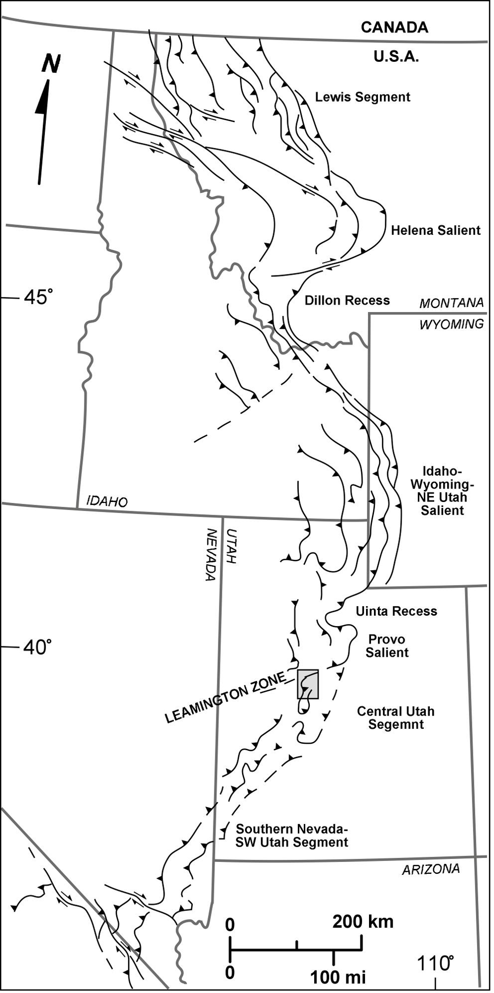
The junction of the Central Utah segment and the Leamington transverse zone is an ideal natural-laboratory for studying salient-recess junctions for several reasons (Figure 1). First, the rocks exposed within the segment continue, uninterrupted, into the transverse zone⁴. So, deformation patterns can be tracked continuously, and compared across the junction. Second, the rocks are essentially monomineralic, so variation in fault patterns are not a result of heterogeneities within units, but instead reflect the overall folding and thrusting within the study area⁴. Third, elastico-frictional mechanisms, such as cataclastic flow, assisted deformation throughout the field area, allowing for direct comparisons of mesoscale fault patterns⁴. Finally, the overall transport direction remained continuous along the length of the segment and transverse zone; therefore, variations in shortening direction did not influence the preserved deformation patterns⁴. All of these factors minimize the number of variables that may have affected the deformation along the segment and transverse zone. As a result, we surmise that the preserved structures formed primarily because of a change in the underlying basement geometry⁵.

Figure 1. Example of index map. The Sevier fold-thrust belt of western USA, showing major salients, segments, recesses and transverse zones. Figure 2 indicated by boxed area (modified from Ismat and Toeneboehn⁷). Please click here to view a larger version of this figure.

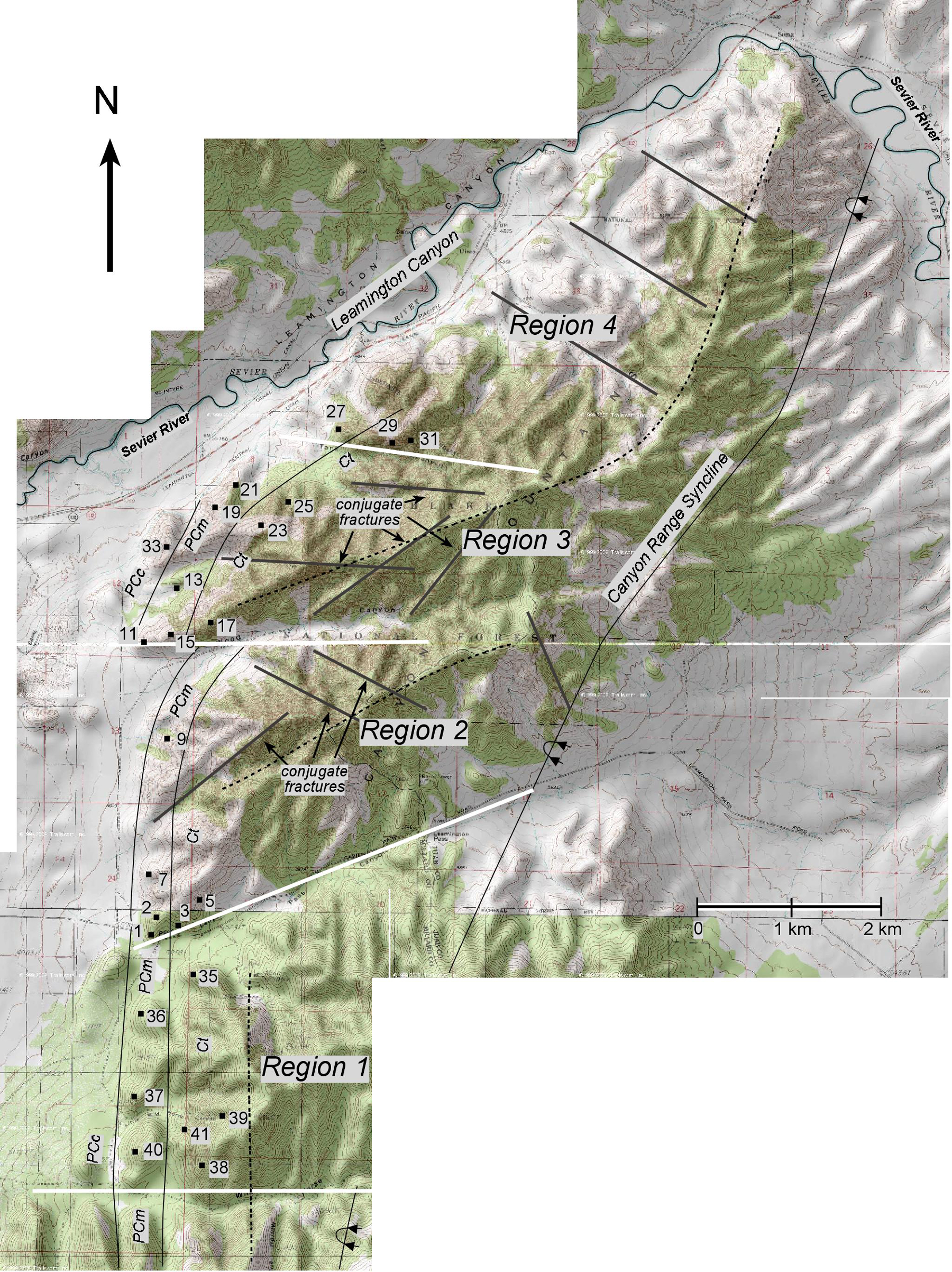
Folding and thrusting within the Central Utah segment and Leamington transverse zone, took place at depths < 15 km, i.e., within the elastico-frictional regime, where deformation occurred primarily by outcrop-scale (< 1 m) faults and cataclastic flow^4,6. Because transport and folding of the thrust sheet took place primarily by elastico-frictional mechanisms, we predict that a detailed fault analysis can provide further insight into the kinematic history of the Leamington transverse zone and the underlying basement geometry. In order to test this hypothesis, we have collected and analyzed fault patterns preserved in the rocks within the northern portion of the Central Utah segment and throughout the Leamington transverse zone (Figure 2).

Figure 2. Example of macroscale topographic map. Shaded-relief topographic map of boxed area in Figure 1. The 4 Regions are separated by solid white lines. Bedding contacts between the Proterozoic Caddy Canyon quartzite (PCc), Proterozoic Mutual quartzite (PCm) and Cambrian Tintic quartzite (Ct) are shown. Dashed lines show the trend of the mountains within this area. Site locations are shown with numbered black squares. First-order lineations are shown with solid gray lines (modified from Ismat and Toeneboehn⁷). Please click here to view a larger version of this figure.

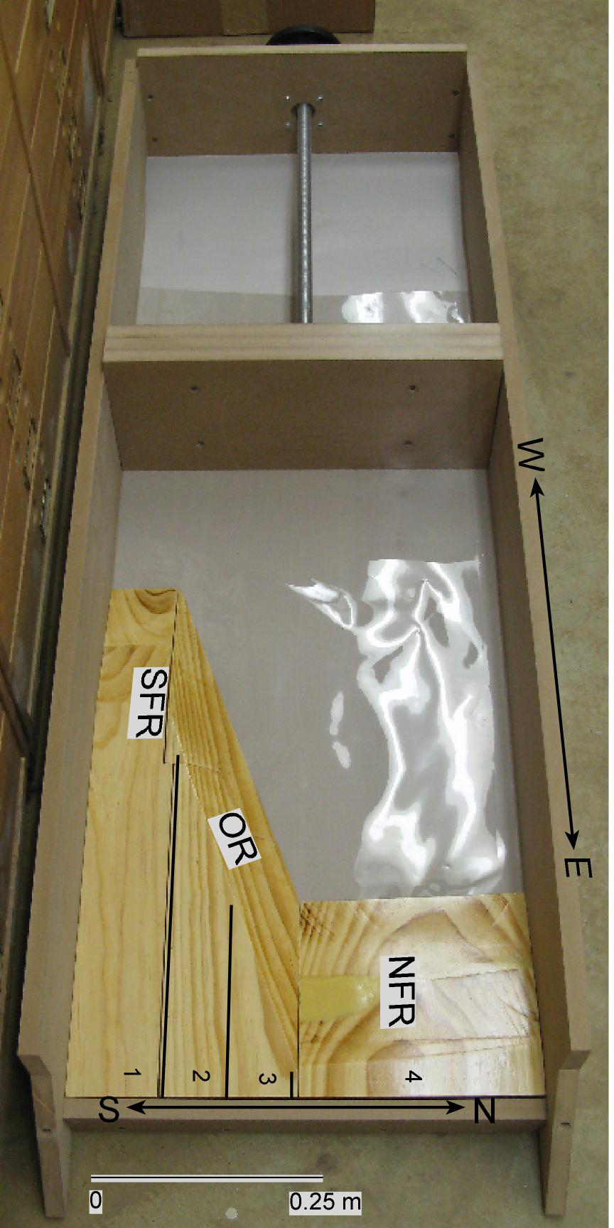
Sandbox experiments were carried out to compare against, and supplement, the fault data. A push-block sandbox model, with frontal and oblique ramps, was used to assist our analyses of the structures preserved in, and around, the Leamington transverse zone (Figure 3) ⁷. The objectives of this approach are four-fold: 1) determine if the mesoscale fault patterns are consistent, 2) determine if the sandbox model supports and explains the field data, 3) determine if the sandbox model provides more details on structures that are not observed in the field, and 4) evaluate whether this combined field-experimental method is useful and easy to replicate.

Figure 3. Example of push-block model. Photograph of empty sandbox model. The southern frontal ramp (SFR), oblique ramp (OR), northern frontal ramp (NFR), and the four Regions (1-4) are labeled (modified from Ismat and Toeneboehn⁷). Please click here to view a larger version of this figure.

Protokół

1. Collection of Macroscale Field Data

1. Before conducting field work, use aerial photographs/topographic maps to identify the overall trend of the mountains (defined by the modern-day ridge crest), transverse zones, faults and other lineations at the macroscale (Figure 2).
   1. Use similar scale topographic maps and aerial photographs, so that patterns can be directly compared. Use 1:24,000 scale maps and photographs.
2. Label and highlight macroscale features on the maps (aerial and/or topographic) to be used in the field. On aerial photographs, use sharp changes in foliage to identify macroscale features, because the foliage patterns reflect the underlying bedrock. On topographic maps, use sharp changes in topography, such as steep cliffs, long narrow valleys and rapid changes in drainage patterns to identify macroscale features.
3. Corroborate these map patterns, with macroscale features found in nature, while in the field. Ensure that the field maps are adjusted accordingly.
4. Subdivide the field area along macroscale transverse zones.

2. Collection of Mesoscale Field Data

1. Conduct field analysis within each transverse zone bound area.
2. Determine the scale of homogeneity of the mesoscale faults throughout the field area. Do this by measuring all faults larger than 3 cm along a transect perpendicular and parallel to the overall macroscale structure. The point at which fault patterns repeat itself along the transect defines the scale of homogeneity.
   Note: 3 cm is chosen as a minimum cut-off because faults smaller than 3 cm may be difficult to measure.
3. Choose representative sites throughout the field area using the defined scale of homogeneity.
   1. Ensure that each site contains ~3 mutually perpendicular rock exposures within the scale of homogeneity, in order to quantify the three-dimensional geometry of the fault work.
   2. Ensure that new sites are chosen where the fault patterns markedly change (Figure 2).
   3. Choose sites far (~one unit of homogeneity) from major bedding contacts, in order to avoid local shortening and elongation directions that may have overprinted faults produced from the overall shortening direction.
4. Use a grid to keep track of all the faults during data collection⁴.
   1. Ensure that the size of the grid is at the scale of homogeneity of the mesoscale faults. For example, if the faults are homogeneous at the cubic meter scale, use a meter square grid.
5. Construct the grid as a collapsible wooden square — this allows for easier transport in the field.
   1. Use 4 equal pieces of 1 in wide strips of wood. Any type of hard wood is recommended because it is the most durable for field work.
   2. Drill 1/4" holes close to the ends (~ ½" from the ends) of the wood strips. Assemble with four 2 1/4" long, 3/16" size screws at each corner. Use steel wing nuts for easiest collapsibility.
   3. Divide the grid equally with string — this helps to track the various faults at each site. Drill holes, equally spaced, along the grids' perimeter, thread and tie string through the holes. For example, for a meter square grid, divide the grid into 10 cm squares with strings connected to the opposite ends of the grid (Figure 4).

Figure 4. Example of a mesoscale outcrop. Bedding is highlighted with white dashed lines. Specific fault sets discussed in paper are highlighted with thin, solid white lines. m² grid is shown (modified from Ismat and Toeneboehn⁷). Please click here to view a larger version of this figure.

6. Make detailed sketches of the fault sets within each grid.
7. Based on the grid sketches and cross-cutting relationships of the faults, determine the youngest fault sets at each site⁴.
   1. Do this by identifying offset fault patterns at each site. The youngest faults overprint and offset the older faults.
8. At each study site, record the orientation, spacing, length, thickness, and morphological characteristics (e.g., healed, vein filled, open, breccia filled) for each of the youngest faults within each grid.
9. Divide the sites amongst the lithologic units (see Figure 2).

3. Collection of Microscale Data

1. Collect oriented rock samples at each site for thin-section analysis.
   1. Ensure that the rock sample is large enough to cut three mutually perpendicular standard size (26 mm x 46 mm) thin-section chips (i.e., slightly larger than an adult fist).
2. Cut thin-section chips (using a standard rock-saw) comparable to the grid orientations from each site, so that the microscale and mesoscale patterns can be directly compared.
3. Prepare standard thickness (0.03 mm) thin-sections⁸.
4. Analyze the thin-sections using a standard optical microscope with an attached camera, for taking photomicrographs.
5. For each thin-section, record morphological characteristics, such as the amount of iron-oxide, and variation and average grain size by using stereological methods, i.e., Spektor Chord analysis (Table 1)⁹.
   1. Do this by measuring the width and/or number of chosen morphological characteristics along 4-6 randomly oriented transects through each thin-section^4,9. From all of the transects, calculate the average (Table 1).

Unit	Bed thickness (m)	Bedding fabric	Grain size (m)	X/Z Fry strain (Average Rf)	X/Y Fry strain (Average Rf)	Amount of overgrowth	Amount of iron oxide	Amount of impurities	Other characteristics
Ct	1,000	Prominent, thick and thin bedded	Ave: 1.59 x 10-4 (Range: 3.6 x 10-6 to 3.31 x 10-4)	1.15	1.12	moderate, semi-connected in small patches	moderate, semi-connected in small patches	moderate, semi-connected calcite in small patches	Ridge former, white to grayish-pink, weathers tan to reddish brown
PCm	570-750	Prominent, well-developed graded and cross-bedding	Ave: 1.48 x 10-4 (Range: 1.15 x 10-4 to 2 x 10-4)	1.22	1.19	major and well-connected	moderate and well-connected	minor calcite and poorly connected	Massive outcrops, purplish red-brown, weathers purple-black

Table 1. Example of microscale morphology. Description of the Proterozoic Mutual (PCm) and Eocambrian Tintic (Ct) quartzite units. X/Z Fry strain is measured in a vertical section parallel to the transport plane, while X/Y Fry strain is measured in a vertical section perpendicular to the transport plane (modified from Ismat and Toeneboehn⁷). Please click here to view/download this table in Microsoft Excel format.

6. Measure strain using normalized Fry analysis^10,11. Ensure that strain is measured from three mutually perpendicular thin-sections in order to determine three-dimensional strain at each site.
   1. Do this by taking a photomicrograph of each thin-section. Ensure that the photomicrographs contain at least 50 grains with solid grain boundaries, i.e., not sub-grain boundaries.
   2. Define the outlines of the grains in order to measure Fry strain. Define the outlines either manually, by tracing the outlines from a printed photomicrograph onto tracing paper, or digitally, by uploading the photomicrograph into an image analysis software program (e.g., Image Pro Plus) that automatically defines the grains' boundaries.
   3. Upload the grain boundary image into the normalized Fry Strain program¹².

4. Plotting Mesoscale Fault Data

1. Analyze the fault data on Equal-area nets. For example, use Stereonet (freeware from R.W. Allmendinger).
   1. Plot the fault sets' poles on Equal-area nets and then contour these poles using 1% area contours (Figure 5).
   2. Determine the most common fault sets from these pole concentrations. Plot these fault sets as great-circles (Figure 5).

Figure 5. Examples of Equal-area plots. Equal-area plots of fault sets from two sites — site 41 is from Region 2 and site 5 is from Region 1. Fault sets are plotted as contoured poles (1% area contours). Average fault sets are determined from pole-concentrations and plotted as great circles. Maximum shortening directions, determined from conjugate-conjugate fault sets, are plotted as black dots. Fault-pole contours are colored according to percentage contribution at each site. Pole concentrations that contribute to >20% are colored red, between 15-19% are colored orange, 10-14% are yellow, 5-9% are green and <5% are colored blue. Red fault-pole contours are labeled as LPS (layer-parallel shortening), LE (limb extension), and HE (hinge-extension) (modified from Ismat and Toeneboehn⁷). Please click here to view a larger version of this figure.

2. Identify the conjugate fault sets, i.e., the great-circle pairs with dihedral angles that range from 40º to 75º (Figure 5)¹³.
3. Define the acute bisector of the conjugate-conjugate fault sets — this locates the maximum shortening direction (Figure 5) ^4,14,15.
4. Further subdivide the equal-area net fault-pole concentrations, according to their percentage contribution for each site. Do this by color coding the pole concentrations, for easier visual analysis. For example, highlight pole concentrations that contribute to >20% of the overall poles for that site red. Color those that contribute between 15-19% orange, 10-14% yellow, 5-9% green and <5% blue (Figure 5, Table 2).

Site	Bedding	Shortening	Highest fault-pole	Fault sets(s)
	(dip, dip direction)	directions(s)	concentration(s)	(dip, dip direction)
		(plunge, trend)	(plunge, trend)
41	83, 268	79, 115	22, 064	68, 244
			60, 345	30, 265
			73, 276	17, 096
5	63, 265	67, 130	08, 343	82, 263
			36, 247	54, 067

Table 2. Example of mesoscale fault data. Chart, showing just 2 of the 24 sites, documenting the following: bedding orientation, shortening direction(s), orientation of the highest fault pole concentration(s) and their corresponding fault set(s) (modified from Ismat and Toeneboehn⁷).

5. Label the pole concentrations according to different fault types (e.g., hinge extension) (Figure 5).
6. Label the different fault types on the mesoscale photos, for easier visual analysis (Figure 4).
7. Graph the different fault types, for easier visual analysis (Figure 6). Do this by graphing the fault data along and across the overall macroscale structure.

Figure 6. Example graph showing distribution of fault populations. Graph showing the percentage and type of the maximum fault sets (highlighted in red in Figure 5) for each site. Just sites within the Ct quartzite are shown here (modified from Ismat and Toeneboehn⁷). Please click here to view a larger version of this figure.

5. Construction of the Push-block Sandbox Model

1. Use ¾ inch MDF (medium-density fiberboard) to reduce potential surface heterogeneities arising from wood grain, coarsely planed surfaces, or other defects from lumber (Figure 3).
2. Apply a basic finishing lacquer to seal the surfaces of the MDF board and prevent epoxy (described below) from permeating the model's surfaces (Figure 3).
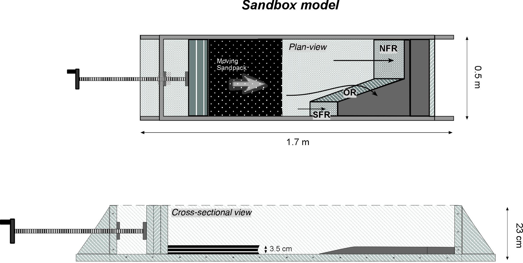
3. Scale and orient the sandbox model to the field area. For example, in this study, model the length of the box to represent the EW trend line, and model the width of the box to represent the NS trend line. Scale the sandbox model where 4 cm is equal to 1 km (Figure 3).
4. Construct the box larger than the field study area in order to avoid potential boundary conditions and/or edge effects from the model.
   1. Do not construct a backstop, in order to allow sand to pass without an unrealistic boundary (Figure 3).
5. Build a push-block equivalent to the width of the sandbox. This will prevent sand from passing through the sides of the push-block.
   1. Use ¾ inch MDF for the push block.
6. Attach the push-block to a crank driven threaded metal bar (Figure 7).
   1. Use a 4-6 inch diameter circular crank with a handle — a circular crank puts less strain on the attendant's wrist and hands.
   2. Use a zinc-plated threaded bar (preferably acme threaded) that is at least ¾ inch in diameter. If the bar is too thin, it may not be able to withstand the weight of the sand.
   3. Ensure that the length of the threaded bar extends from the beginning of the sandbox to the end of the ramps.

Figure 7. Example sandbox model diagram. Diagrams for the sandbox model, illustrated as plan and cross-sectional views. The southern frontal ramp (SFR), oblique ramp (OR) and northern frontal ramp (NFR) are labeled. Thin arrows drawn over the ramps illustrate potential direction of sand movement. See Figure 3 for a photograph of an empty sandbox model (modified from Ismat and Toeneboehn⁷). Please click here to view a larger version of this figure.

7. Drill an elongated hole, with a vertical long axis, in the center of the frontstop. This elongated shape will allow the push-block (attached to the threaded bar) to move up and over the ramps, if needed (Figure 8).
   1. Ensure that the length of the elongated hole is equal to the height of the tallest ramp.
   2. Secure the elongated hole with a metal frame. Attach the metal frame to the frontstop with nuts and bolts (Figure 8).
   3. Thread the rod through a matching pitch and diameter nut mounted to the frontstop (Figure 8).

Figure 8. Example threaded bar connection. Close-up view of the threaded bar and matching nut mounted to the frontstop. Please click here to view a larger version of this figure.

8. Construct an oblique ramp, bound on both sides by frontal ramps. Construct the ramps out of pine with glued rabbet joints on the top surfaces and countersunk fasteners along the base.
   1. Cut the ramps at comparable orientations to what is predicted in the field.
   2. Expand the distance between the various ramps, as compared to what is observed in the field, so that the structures that form in the sand are more visible.
9. Sand the surfaces with a fine grit sanding paper to remove surface heterogeneities and apply a polyurethane finish to protect the soft wood.
10. Cover the ramps and the base of the sandbox with painters tape to protect the wood from epoxy between trials. Ensure that the tape is smooth and free from ridges or flaps.

6. Running the Push-block Sandbox Model

1. Use typical play-sand. This type of sand is relatively homogeneous, with an average grain size of 0.5 mm.
2. Dye and dry half of the sand.
   1. Fill a 5-gallon bucket a quarter full with play-sand and add black food coloring while mixing until a uniform dark green color is attained. Use as much dye as is needed to make the color of the dyed sand clearly distinctive from the undyed sand.
   2. Allow sand to dry at room temperature, which may take several days, or in an oven (up to 500 ºC), which may only take a few hours. Do not place hot sand in the sandbox. Ensure that the sand has cooled to room temperature before use.
3. Lay the sand in alternating layers of colored and uncolored (tan) sand. Test various thicknesses of sandpacks. In this set-up, the clearest and most reproducible results were produced with a sandpack 3.5 cm thick, with alternating colored and tan layers 0.6 cm thick (Figure 7).
4. Gently press a plastic mesh, composed of 0.5 in² (1.3 cm²) squares onto the top of the undeformed sand to produce a grid indentation (Figure 9).

Figure 9. Example of undeformed sand in sandbox model. Partial plan-view of undeformed sand in sandbox model. Note grid indentation and square cross-pins. The southern frontal ramp (SFR), oblique ramp (OR), northern frontal ramp (NFR), and the four Regions (1-4) are labeled (modified from Ismat and Toeneboehn⁷). Please click here to view a larger version of this figure.

5. Insert square cross pins 2 inches (~5 cm) apart throughout the undeformed sand (Figure 9).
6. Push the sand with the crank driven push-block. In this set-up, move the sand 60 cm, i.e., 60 cm of shortening (Figure 10).
   1. Move the push-block slow enough so that changes in the sand can be carefully documented. The speed at which the push-block is moved (i.e., strain rate) does not affect the results.
   2. Track the deformation by observing the shape changes of the squares (Figure 10).
   3. Track the amount of transport and vertical rotation by observing the motion of the pins (Figure 10).
   4. Document all of these changes with a camera mounted near the sandbox, so that the entire sandbox is within the picture field. Ensure to take still frame photographs as well as videos.

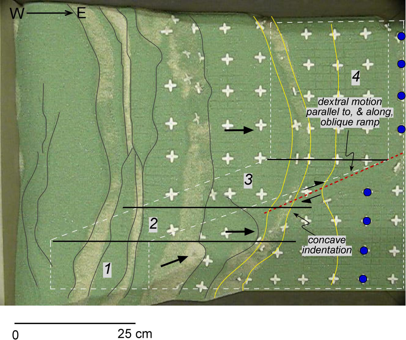
Figure 10. Example of deformed sand layers. Plan-view of the end-result deformation from the sandbox model. Select cross-pins labeled with blue dots showing dextral offset. Folded cross-pins highlighted with yellow lines. Thrust faults are highlighted with thin, black lines. The four Regions (1-4) are labeled (modified from Ismat and Toeneboehn⁷). Please click here to view a larger version of this figure.

7. Experiment with varying amounts of sand and total shortening.
   1. Repeat until satisfied, i.e., until the structures formed in the sandbox mimic those preserved in nature, under comparable shortening amounts.

7. Collecting Samples from the Sandbox

1. Remove all cross-pins from the sand once the sandbox results mimic those preserved in nature.
2. Collect samples from the sandbox by separating and epoxying portions of the deformed sand (Figure 11).
   1. Do this by constructing two pre-cut sheet-metal dividers to isolate portions of the deformed sand (Figure 9).
   2. Ensure that the bottom edge of the divider is cut to match the angle of the ramp.
   3. To protect the dividers from epoxy between trials, cover the dividers with painters tape (Figure 11).
   4. Ensure that the dividers extend over and beyond the ramps. In this study, use rectangular dividers that measured 45 cm long and 9 cm wide (Figure 11).
   5. Ensure that the dividers are taller than the thickest portion of the deformed sandpack (Figure 11).
   6. Ensure that one end of the divider is closed, in order to control the flow of the epoxy. Do not close the other end of the divider, in order to minimize any potential disturbance to the sandpack (Figure 11).

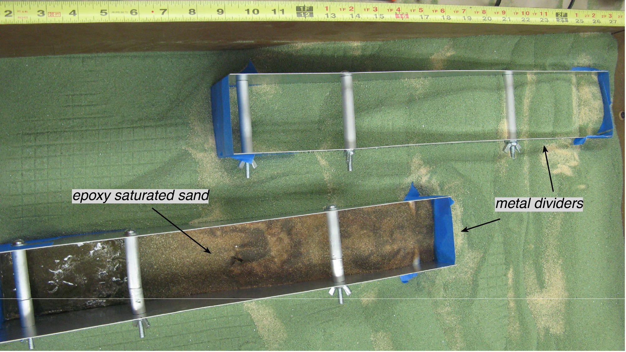
Figure 11. Example of metal dividers. Plan-view, showing 2 metal dividers, one through a frontal ramp and one through the oblique ramp, in the deformed sand. The metal divider along the oblique ramp is filled with epoxy. Note tape measure for scale (Modified from Ismat and Toeneboehn⁷). Please click here to view a larger version of this figure.

3. Steady the dividers with metal bars (Figure 11).
   1. Do this by fastening the dividers with ¼ inch x 4 inch machine screws through pre-drilled holes toward the top of the dividers. Sheath the screws with 3/8 inch diameter aluminum tubing between the divider's sides. In this study, use two metal bars for each divider (Figure 11).
4. Place one divider on the oblique ramp, and the second on the frontal-oblique ramp junction (Figure 11).
5. Pour warmed epoxy across the top of the sand portions isolated by the metal dividers (Figure 11).
   1. Continue to pour epoxy until it is no longer absorbed by the sand. This ensures that the sand is fully saturated.
6. Pull the epoxied areas out of the metal dividers, once the epoxy is dry. Do this by pulling the dividers out with the metal bars.
7. Using a rock saw, cut the epoxied areas perpendicular and parallel to the strike of the ramps.
8. Highlight the bedding, folds and faults with a permanent marker on the epoxied samples (Figure 12).

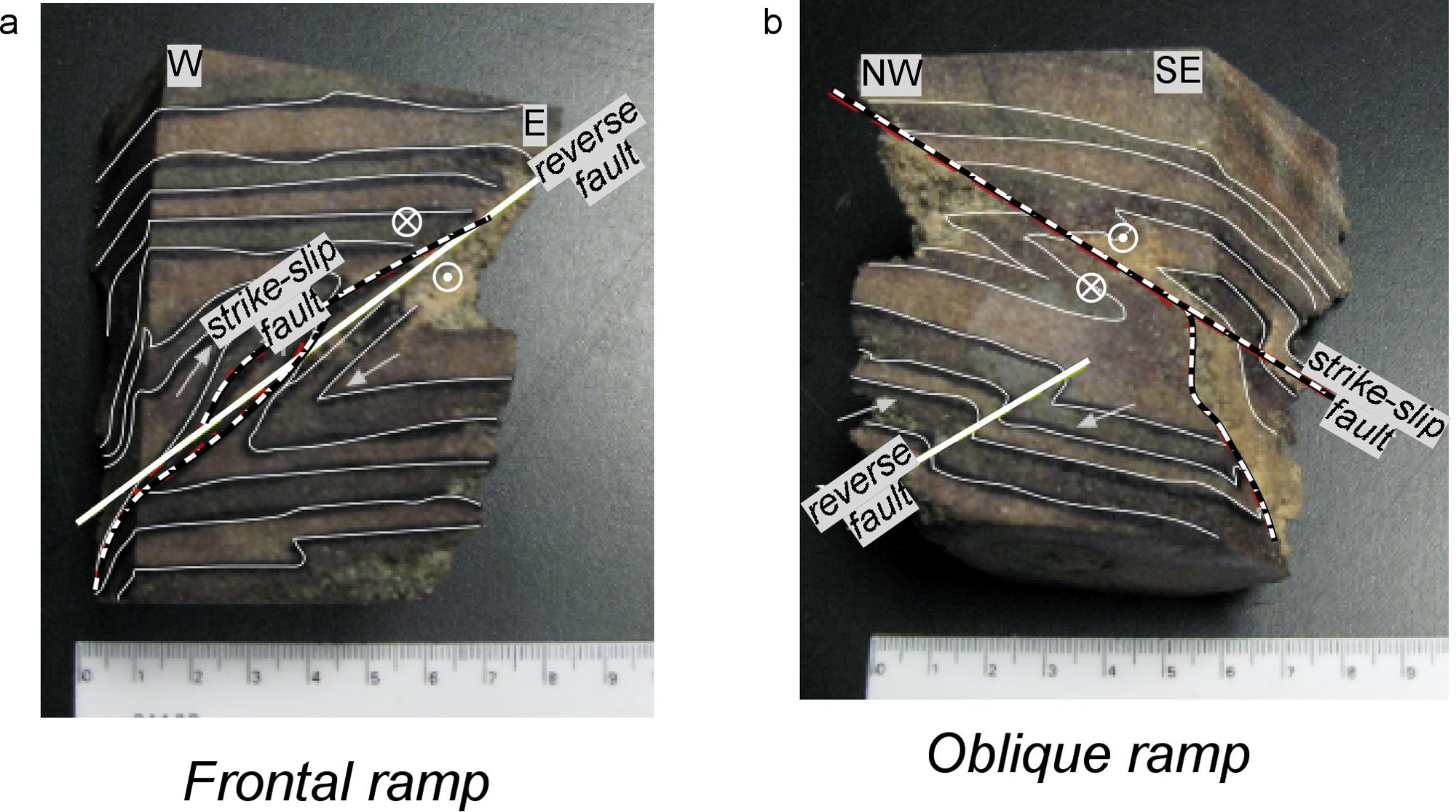
Figure 12. Examples epoxied samples from sandbox model. Epoxied samples from the (a) northern frontal ramp and the (b) oblique ramp within the sandbox model. Shown samples are cut perpendicular to the trend of the ramps. Layers are highlighted with thin, white lines. Solid white lines mark reverse faults, dashed white lines mark strike slip faults (modified from Ismat and Toeneboehn⁷). Please click here to view a larger version of this figure.

9. Compare the sandbox samples to the field data.
   1. Compare samples with cross-sections from the area. Be sure the samples and cross-sections have similar orientations.

Wyniki

Aerial photographs were used to subdivide the field area into four Regions (1-4), based on the trend of the modern mountain ridge crest (Figure 2). Multi-scale fault data is compared between these four Regions. Assuming that these trend changes reflect the underlying basement geometry, the oblique ramp is positioned within Regions 2 and 3, where the mountains trend oblique to the Sevier fold-thrust belt. Throughout the four Regions, we found that the mesoscale faults pres...

Dyskusje

The Central Utah segment of the Sevier fold-thrust belt, and its northern boundary, the Leamington transverse zone serves as an ideal natural laboratory for studying salient-recess junctions (Figure 1). Along this junction, the transport direction remains constant and the thrust sheets are uninterrupted across the junction, so the only variable is the underlying basement geometry⁵.

Here, we present a method to analyze this type of salient-recess junction by combinin...

Materiały

Name	Company	Catalog Number	Comments
fiberboard	Any	NA
finishing lacquer	Any	NA
epoxy	Epoxy technology	Parts A and B: 301-2 2LB	Best if warmed to 80º - 125º. If warming is not possible, it will cure fine, it will just take 1 week, rather than 1 day.
ramp wood-pine	Any	NA
painters tape	Any	NA
rabbit joints	Any	NA
countersunk fasteners	Any	NA
sand paper	Any	NA
play sand	Any	NA	best if homogenous grain size, ~0.5 mm
food coloring	Any	NA	best to use one color and a dark color
plastic mesh/grid	Any	NA
square cross oins	Any	NA
crank screw	Any	NA
crank handle	Any	NA
sheet metal	Any	NA
dividers bars	Any	NA