1. Relative Permeability Identification
Follow the procedure to find the relative permeability of the small inductor (yellow/white ferrite core). The core dimensions are shown in Fig. 2, and the number of turns is N=75.
- Using a LCR meter, measure the inductance of the inductor at both 120 Hz and 1000 Hz.
- Build the circuit in Fig. 1 on a proto-board, but keep the function generator output disconnected from the proto-board.
- Check a differential voltage probe and a current probe for no offsets with the current probe connected on channel 1 and the voltage probe connected on channel 2.
- Note the scaling factors for the differential probe on the probe itself and on the scope. Set the differential probe to 1/20 for a better resolution.
- Set the current probe to 100 mV/A on the probe itself and 1X on the scope. Remember that these scaling factors need to be used when performing calculations.
- Set the function generator output (50 Ω BNC output connector) at 10 V peak and 1000 Hz sinusoidal waveform. Observe the waveform using the differential voltage probe.
- Leave the function generator on even when disconnected, but avoid shorting its terminals. Turning the function generator off resets many settings.
- Connect the current and voltage probes to measure vC and i.
- Check that the circuit is as desired and that all connections are maintained.
- Connect the function generator to the circuit.
- Take a screenshot of the measured current and voltage with at least three periods shown in addition to the peak or RMS values of the measured signals.
- From the "Display" menu on the scope, change the display format from "YT" to "XY".
- Observe the B-H curve by adjusting the channel 1 and channel 2 vertical adjustment knobs until the curve fits the scope screen.
- In order to see a steadier curve, use the "persist" option from the display menu at a setting of 1 or 2 s.
- Take a screenshot of the measured B-H curve.
- Adjust the function generator frequency to 120 Hz and retake the B-H curve screenshot after adjusting the curve settings as needed.
- Disconnect the function generator and remove the inductor. Keep the rest of the circuit intact.
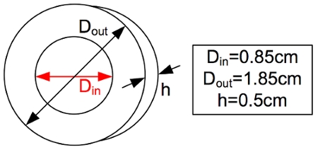
Figure 2: Dimensions of the smaller inductor core. Please click here to view a larger version of this figure.
2. Identifying the Number of Turns
The larger black inductor (Bourns 1140-472K-RC) has an unknown number of turns. To simplify calculations, assume the core to be an all-air-core solenoid with a radius of 1.5 cm and length of 2.5 cm. If this assumption is not taken, the geometry of the core will have to be considered and will complicate calculations. However, this assumption is still reasonable given that with a solenoid, flux has to pass through air on both sides of the device and air is the dominant flux path medium.
- Using the LCR meter, measure the inductance of the provided inductor at both 120 Hz and 1000 Hz.
- Place the inductor in the circuit shown in Fig. 1 , which should still be intact from the previous part of the experiment.
- Check a differential voltage probe and a current probe for no offsets with the current probe connected on channel 1 and the voltage probe connected on channel 2.
- Note the scaling factors for the differential probe on the probe itself and on the scope. Set the differential probe to 1/20 for a better resolution.
- Set the current probe to 100 mV/A on the probe itself and 1X on the scope. Remember that these scaling factors need to be used when doing calculations utilizing any measurements or data captures for further analysis.
- Set the function generator output (50 Ω BNC output connector) at 10 V peak and 1000 Hz sinusoidal waveform. Observe the waveform using the differential voltage probe.
- Leave the function generator on even when disconnected, but avoid shorting its terminals. Turning the function generator off resets many settings.
- Connect the current and voltage probes to measure vC and i.
- Check the circuit, and make sure that connections are as desired.
- Connect the function generator to the circuit.
- Take a screenshot of the measured current and voltage with at least three periods shown in addition to the peak or RMS values of the measured signals.
- From the "display" menu on the scope, change the display format from "YT" to "XY".
- Observe the B-H curve by adjusting the channel 1 and channel 2 vertical adjustment knobs until the curve fits the scope screen.
- In order to see a steadier curve, use the "persist" option from the display menu at a setting of 1 or 2 s.
- Take a screenshot of the measured B-H curve.
- Adjust the function generator frequency to 120 Hz and retake the B-H curve screenshot after adjusting the curve settings as needed.
- Turn off the function generator and disassemble the circuit.
3. B-H Curve of a 60 Hz Transformer
The transformer used in this demonstration steps down 115 V RMS to 24 V RMS, but can only be used for B-H curve characterization in this experiment, thus only the 120 V RMS terminals are used. The transformer dimensions are shown in Fig. 3.
- Using the LCR meter, measure the inductance of the 115 V-side winding at 120 Hz (closer to the rated 60 Hz).
- Make sure the three-phase disconnect switch is in the off position.
- Connect the three-phase cable to the VARIAC.
- Build the circuit shown in Fig. 4. Have the transformer sit on the side of the proto-board. Use banana cables to connect AC1 and N from the VARIAC to the proto-board.
- Make sure the VARIAC is set at 0%.
- Check a differential voltage probe and a current probe for no offsets with the current probe connected on channel 1 and the voltage probe connected on channel 2.
- Note down the scaling factors for the differential probe on the probe itself and on the scope. Set the differential probe scaling to 1/200.
- Set the current probe to 100 mV/A on the probe itself and 1X on the scope. Remember that these scaling factors need to be used when doing calculations.
- Connect the current and voltage probes to measure vC and i.
- Check the circuit.
- Turn on the three-phase disconnect switch, and slowly adjust the VARIAC until 90% is reached.
- Take a screenshot of the measured current and voltage with at least three periods shown in addition to the peak or RMS values of the measured signals.
- From the "Display" menu on the scope, change the display format from "YT" to "XY".
- Observe the B-H curve by adjusting the channel 1 and channel 2 vertical adjustment knobs until the curve fits the scope screen.
- In order to see a steadier curve, use the "persist" option from the display menu at a setting of 1 or 2 s.
- Take a screenshot of the measured B-H curve.
- Restore the VARIAC to 0%, turn the disconnect switch off, and disassemble the circuit.
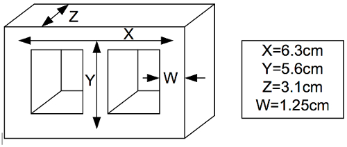
Figure 3: Dimensions of the transformer core. Please click here to view a larger version of this figure.
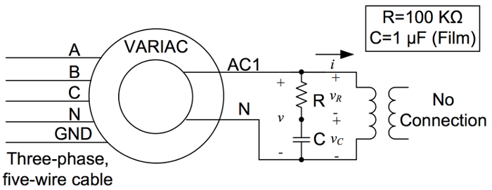
Figure 4: Test circuit to determine the B-H curve of a 60 Hz transformer. Please click here to view a larger version of this figure.
 (7)
(7)


