
Determination of Impingement Forces on a Flat Plate with the Control Volume Method
Genel Bakış
Source: Ricardo Mejia-Alvarez and Hussam Hikmat Jabbar, Department of Mechanical Engineering, Michigan State University, East Lansing, MI
The purpose of this experiment is to demonstrate forces on bodies as the result of changes in the linear momentum of the flow around them using a control volume formulation [1, 2]. The control volume analysis focuses on the macroscopic effect of flow on engineering systems, rather than the detailed description that could be achieved with a differential analysis. Each one of these two techniques have a place in the toolbox of an engineering analyst, and they should be considered complementary rather than competing approaches. Broadly speaking, control volume analysis will give the engineer an idea of the dominant loads in a system. This will give her/him an initial feeling about what route to pursue when designing devices or structures, and should ideally be the initial step to take before pursuing any detailed design or analysis via differential formulation.
The main principle behind the control volume formulation is to replace the details of a system exposed to a fluid flow by a simplified free body diagram defined by an imaginary closed surface dubbed the control volume. This diagram should contain all surface and body forces, the net flux of linear momentum through the boundaries of the control volume, and the rate of change of linear momentum inside the control volume. This approach implies cleverly defining the control volume in ways that simplify the analysis at the same time that capture the dominant effects on the system. This technique will be demonstrated with a plane jet impinging on a flat plate at different angles. We will use control volume analysis to estimate the aerodynamic load on the plate, and will compare our results with actual measurements of the resulting force obtained with an aerodynamic balance.
Prosedür
1. Setting the facility
- Make sure that there is no flow in the facility.
- Connect the positive port of the pressure transducer to the plenum pressure tap (
 ).
). - Leave the negative port of the pressure transducer open to the atmosphere (
 ).
). - Record the transducer's conversion factor from Volts to Pascals (
 ).
). - Record the
Sonuçlar
Figure 3 shows a comparison between the normal load on the flat plate as measured directly from an aerodynamic balance and estimated from conservation of linear momentum. In general, the analysis of linear momentum captured the dominant tendency of direct measurements as the impingement angle changes. The discrepancies in these measurements varied non-monotonically with the impingement angle. For impingement angles in the range
Log in or to access full content. Learn more about your institution’s access to JoVE content here
Başvuru ve Özet
We demonstrated the application of control volume analysis of conservation of linear momentum to determine the forces exerted by a jet impinging on a flat plate. This analysis proved simple to apply, and gave a satisfactory bulk estimation of loads without requiring detailed knowledge of the flow pattern around the plate. Though there were some discrepancies (both in magnitude as well as tendency) due to the basic assumption of inviscid transformation of momentum, this technique offers a means of obtaining a quick estima
Referanslar
- White, F. M. Fluid Mechanics, 7th ed., McGraw-Hill, 2009.
- Munson, B.R., D.F. Young, T.H. Okiishi. Fundamentals of Fluid Mechanics. 5th ed., Wiley, 2006.
- Buckingham, E. Note on contraction coefficients of jets of gas. Journal of Research,6:765-775, 1931.
- Lienhard V, J.H. and J.H. Lienhard IV. Velocity coefficients for free jets from sharp-edged orifices. ASME Journal of Fluids Engineering, 106:13-17, 1984.
Etiketler
 ; vertical force:
  ).
). ).
).
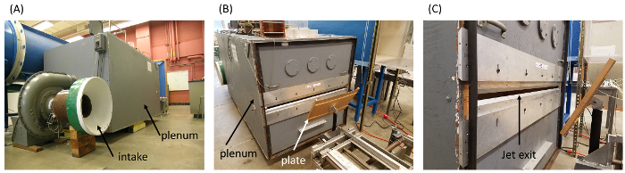
 . (B): discharge side with impingement plate. (C): Detail of discharge slit.
 Atla...
Bu koleksiyondaki videolar:

Now Playing
Determination of Impingement Forces on a Flat Plate with the Control Volume Method
Mechanical Engineering
26.0K Görüntüleme Sayısı

Buoyancy and Drag on Immersed Bodies
Mechanical Engineering
30.1K Görüntüleme Sayısı

Stability of Floating Vessels
Mechanical Engineering
22.8K Görüntüleme Sayısı

Propulsion and Thrust
Mechanical Engineering
21.9K Görüntüleme Sayısı

Piping Networks and Pressure Losses
Mechanical Engineering
58.6K Görüntüleme Sayısı

Quenching and Boiling
Mechanical Engineering
7.7K Görüntüleme Sayısı

Hydraulic Jumps
Mechanical Engineering
41.1K Görüntüleme Sayısı

Heat Exchanger Analysis
Mechanical Engineering
28.0K Görüntüleme Sayısı

Introduction to Refrigeration
Mechanical Engineering
24.9K Görüntüleme Sayısı

Hot Wire Anemometry
Mechanical Engineering
15.7K Görüntüleme Sayısı

Measuring Turbulent Flows
Mechanical Engineering
13.6K Görüntüleme Sayısı

Visualization of Flow Past a Bluff Body
Mechanical Engineering
12.0K Görüntüleme Sayısı

Jet Impinging on an Inclined Plate
Mechanical Engineering
10.8K Görüntüleme Sayısı

Conservation of Energy Approach to System Analysis
Mechanical Engineering
7.4K Görüntüleme Sayısı

Mass Conservation and Flow Rate Measurements
Mechanical Engineering
22.8K Görüntüleme Sayısı
JoVE Hakkında
Telif Hakkı © 2020 MyJove Corporation. Tüm hakları saklıdır