Frequency Mixing Magnetic Detection Scanner for Imaging Magnetic Particles in Planar Samples

Summary

A scanner for imaging magnetic particles in planar samples was developed using the planar frequency mixing magnetic detection technique. The magnetic intermodulation product response from the nonlinear nonhysteretic magnetization of the particles is recorded upon a two-frequency excitation. It can be used to take 2D images of thin biological samples.

Abstract

The setup of a planar Frequency Mixing Magnetic Detection (p-FMMD) scanner for performing Magnetic Particles Imaging (MPI) of flat samples is presented. It consists of two magnetic measurement heads on both sides of the sample mounted on the legs of a u-shaped support. The sample is locally exposed to a magnetic excitation field consisting of two distinct frequencies, a stronger component at about 77 kHz and a weaker field at 61 Hz. The nonlinear magnetization characteristics of superparamagnetic particles give rise to the generation of intermodulation products. A selected sum-frequency component of the high and low frequency magnetic field incident on the magnetically nonlinear particles is recorded by a demodulation electronics. In contrast to a conventional MPI scanner, p-FMMD does not require the application of a strong magnetic field to the whole sample because mixing of the two frequencies occurs locally. Thus, the lateral dimensions of the sample are just limited by the scanning range and the supports. However, the sample height determines the spatial resolution. In the current setup it is limited to 2 mm. As examples, we present two 20 mm × 25 mm p-FMMD images acquired from samples with 1 µm diameter maghemite particles in silanol matrix and with 50 nm magnetite particles in aminosilane matrix. The results show that the novel MPI scanner can be applied for analysis of thin biological samples and for medical diagnostic purposes.

Introduction

Magnetic nanoparticles (MNP) have found widespread applications in molecular biology and in medicine, i.e., for manipulation of biomolecules and single cells¹, for selectively labeling target entities for detection,^{2, 3} for chromatin modulation,⁴ and for mRNA isolation and cancer treatment.⁵ Due to their superparamagnetic properties, they are especially useful for medical imaging. They can serve, for instance, as contrast agents or tracers for Magnetic Resonance Imaging (MRI) or for susceptibility imaging using Superconducting Quantum Interference Device (SQUID) detectors. ^{2, 6} The superparamagnetic nanoparticles yield a good contrast to the different tissues of the human body which are dia- or paramagnetic.⁷ Thus, the particles can conveniently be used to acquire medical images of human body parts with relatively good spatial resolution and sensitivity.⁸

The Magnetic Particle Imaging (MPI) technique introduced by Gleich and Weizenecker⁹ makes use of the nonlinearity of the particle's magnetization. At zero or weak magnetic field bias, the response of MNP to an ac excitation of frequency f is strong due to their large susceptibility. In particular, the particle's nonlinear magnetization gives rise to the generation of harmonics n·f, with n = 2, 3, 4 … At high magnetic field bias, the harmonic response becomes weak because the particles are magnetically saturated. In the MPI technique, the sample is completely magnetized except for a field-free line (FFL) or a field-free point (FFP). Only particles situated close to this line or point will contribute to the nonlinear response of the sample. With the movement of a FFP and employment of suitable receiver coils, Gleich and Weizenecker acquired MPI images with a spatial resolution of 1 mm.

In order to obtain information on the spatial distribution of MNP, two methods are usually employed, the mechanical movement of the sensor with respect to the sample, or movement of the FFL/FFP by means of electromagnets.^{2, 3} In the latter case, image reconstruction techniques like harmonic-space MPI³ or X-space MPI^{10, 11, 12} are required. The spatial resolution of MPI is determined by the convolution properties of excitation and detection coils as well as by the characteristics of the magnetic field gradient. This allows image reconstruction algorithms to obtain an improved resolution over the native resolution, which is determined by size and distance of the pickup coils as well as by the magnetic field distribution governed by Maxwell's equations.

A MPI scanner is usually comprised of a strong magnet for magnetizing the whole sample, a controllable coil system for steering a FFL or FFP across the sample, a high frequency excitation coil system, and a detection coil system for picking up the nonlinear response from the sample. The FFL/FFP is continuously moved through the sample volume while the harmonic response from this unsaturated sample region is recorded. In order to avoid the problem of fitting the specimen into the scanner, a single-sided MPI scanner has been demonstrated by Gräfe et al.¹³, however at the expense of reduced performance. Best results are obtained if the sample is surrounded by the magnets and coils. Because the sample has to be fully magnetized except for the FFL/FFP region, the technique requires relatively large and strong magnets with water cooling, leading to a rather bulky and heavy MPI system.

Our approach is based on frequency mixing at the non-linear magnetization curve of superparamagnetic particles.¹⁴ When super-paramagnets are exposed to magnetic fields at two distinct frequencies (f₁ and f₂), sum frequencies representing a linear combination m·f₁ + n·f₂ (with integer numbers m, n) are generated. It was shown that the appearance of these components is highly specific to the nonlinearity of the magnetization curve of the particles.¹⁵ In other words, when the MNP sample is simultaneously exposed to a driving magnetic field at frequency f₂ and a probing field at frequency f₁, the particles generate a response field at frequency f₁ + 2·f₂. This sum frequency would not be existent without the magnetically nonlinear sample, therefore the specificity is extremely high. We called this method "frequency mixing magnetic detection" (FMMD). It has been experimentally verified that the technique yields a dynamic range of more than four orders of magnitude in particle concentration.¹⁴

In contrast to typical MPI instrumentation, the planar frequency mixing magnetic detection (p-FMMD) approach does not require to magnetize the sample close to saturation because the generation of the sum frequency component f₁ + 2·f₂ is maximum at zero static bias field.¹⁴ Therefore, the need for strong and bulky magnets is alleviated. In fact, the outer dimensions of the measurement head are only 77 mm × 68 mm × 29 mm. For comparison, MPI setups are typically meter-sized.⁷ The drawback, however, is that the technique is restricted to planar samples with a maximum thickness of 2 mm in the current setup. The sample has to be scanned relatively to the two-sided measurement head. A re-construction allowing for thicker samples is possible, but has to be traded in for a loss of spatial resolution.

Based on this FMMD technique, we present a special type of MPI detector for planar samples, the so-called "planar frequency mixing magnetic detection" (p-FMMD) scanner. The principle has been recently published.¹⁷ In this work, we focus on the methodology of the technique and present protocols how to set up such a scanner and how to perform scans. It has been shown that MPI can be applied for medical diagnostic purposes such as cardiovascular or cancer imaging.^{16, 18, 19} Therefore we believe that the new MPI scanner can be used for a broad range of potential applications, e.g., for measuring magnetic particle distribution in tissue slices.

Access restricted. Please log in or start a trial to view this content.

Protocol

1. Design a Planar FMMD Measurement Head

1. Choose a coil scheme for the measurement head. Select a configuration according to Figure 1, consisting of two pickup coils above and two below the sample in a (-, +, +, -) sequence, with the sample sitting in the center between the two (+) coils. The sign denotes the direction of winding, i.e., (+) for clockwise and (-) for counterclockwise. Thus, the sensitivity of the pickup coils becomes almost homogeneous across the sample thickness.
   1. Place the excitation coils such that the directly induced signal in the pickup coils cancels out in order to prevent saturation of the preamplifier and achieve maximum sensitivity to the sample. Other configurations that fulfill these basic design rules can be devised.
2. Specify the maximum sample thickness. Here, use 2 mm.
   1. Choose the diameter and length of the pickup coils similar to the maximum sample thickness. Here, an inner diameter of 2 mm was chosen, which yields an average diameter of 3.7 mm for the height of windings of 1.7 mm. The coil width is 4 mm.
   2. Choose the wire diameter and the number of windings of the pickup coils such that the total impedance of all pickup coils approximately matches the input impedance of the preamplifier. This condition imposes restrictions on the detection frequency. In the case of a operational amplifier with an optimum input impedance of 1,100 Ω, all four pickup coils have 600 windings of 0.08 mm dia. enameled copper wire, yielding a total Ohmic series resistance of 95.3 Ω and a total inductance of 1.9 mH, which gives 919 Ω impedance.
3. Prepare the high frequency excitation coils¹⁷ such that the magnetic field at the sample's location ideally amounts to about 0.5 mT. For instance, if the inner radius of the coil is 3.8 mm and the width is 8.5 mm, wind 476 windings of 0.1 mm diameter wire. Here, a field of 0.4 mT was achieved at f₁ = 76,550 Hz.
4. Prepare the low frequency excitation coils¹⁷ such that the magnetic field at the sample's location is about 5 mT. For instance, if the inner radius of the coil is 5 mm and the width is 8.5 mm, wind 2,000 windings of 0.12 mm diameter wire. The setup yielded 5 mT at f₂ = 61 Hz.

Figure 1. Schematic drawing of the p-FMMD set-up. Two measurement heads are electronically connected to each other. The sample is placed in the space between the heads. Detection coils (+) measure the sample signal, counter-wound detection coils (-) serve as reference to cancel out the direct field from the high frequency excitation coils. Amp - preamplifier, x - mixer, LPF - low pass filter, DAQ - data acquisition. Please click here to view a larger version of this figure.

2. Construct the Measurement Head

1. Construct the p-FMMD such that two sets of excitation and detection coils are attached above and below the sample. Each set of coils consists of a low frequency driver coil, a high frequency excitation coil, and a differential detection coil comprising two oppositely wound pickup coils in axial gradiometer configuration.
   1. Allow for an adjustability of at least one excitation coil relative to the differential detection coil in order to be able to balance out direct induction of the high frequency excitation into the detection coil. For instance, mount the excitation coil on a thread which allows relative movement of the excitation coil versus the detection coil. A schematic diagram of the p-FMMD is shown in Figure 1. Figure 2 depicts a technical drawing and a photograph of the setup. Detailed parameters of the coils are listed in Table 1.
2. Mount the coil sets above and below the sample on a rigid support, with coaxial orientation, see Figures 1 and 2. Make sure that the two coil sets do not vibrate relative to each other.
3. Adjust the high frequency balance of the measurement head by applying the high frequency excitation current to the respective excitation coil set, varying the relative position between them, and simultaneously measuring the detected signal at this frequency at the detection coil set, using equipment such as an oscilloscope or a lock-in amplifier.
   1. Adjust the directly induced voltage as low as a few millivolts, i.e., more than 1,000-fold suppression of direct induction. Determine the limit of adjustability by observing the phase shift between excitation current and detected voltage. At the minimum, the induced voltage is 90° phase-shifted as compared to direct induction.

Figure 2. Technical drawing and photo of p-FMMD head. Cross-sections along a vertical plane (top left) and a horizontal plane (bottom left) are shown as well as a photograph of the opened measurement head before coil winding. 1 - Aluminum support, 2 - coil former for detection coils, 3 - threaded coil former for excitation coils which can be moved up/down by rotation, 4 - sample support plates, 5 - aluminum lids, 6 - sample stopper support, 7 - stopper in x direction, 8 - stopper in y direction. 6 - 8 are removed for scanning. The size of the p-FMMD head is 77 mm × 68 mm × 29 mm. Please click here to view a larger version of this figure.

3. Set up Measurement Electronics

1. Configure the excitation section, consisting of the two oscillators and power amplifiers for both low frequency driver coil and high frequency excitation coil.
   1. Set up the low frequency driver section, comprising an oscillator and a power amplifier for the low frequency f₂. Calculate the power of the amplifier such that it delivers the required current to produce the field of about 5 mT in the driver coil. Here, use a Direct Digital Synthesis (DDS) chip as programmable oscillator. Employ a high-speed buffer as power amplifier.
   2. Set up the high frequency excitation section, comprising an oscillator and a power amplifier for the high frequency f₁. Set up the power amplifier such that it delivers the required current to produce the field of about 0.5 mT in the excitation coil. Use a DDS chip and a high-speed buffer as oscillator and power amplifier, respectively.
2. Configure the detection section, consisting of a preamplifier, a first mixer to demodulate from the high frequency f₁, an intermediate amplifier and filter, a second mixer to demodulate from twice the low frequency 2·f₂, and a final filter and output driver. Alternatively, use two lock-in amplifiers to implement the detection electronics.
   1. Set up the preamplifier stage. Select the input operational amplifier (OP), considering the impedance of the detection coil and the gain-bandwidth product. Perform the noise optimization procedure, taking into account the specified voltage noise and current noise of the OP, as explained in Ref. 10. Select a high-speed low-noise operational amplifier with an amplification of about 100 in the first stage. The subsequent stage is uncritical, but check that the output signal remains in the voltage range, i.e., not distorted due to overloading. Here, use a low-noise JFET input operational amplifier with 4.3-fold amplification.
   2. Set up the first demodulation stage, multiplying the amplified signal with the high frequency f₁. Use an analog multiplier chip and reference it from a second separate DDS chip in order to realize an adjustable phase for demodulation. Alternatively, use a lock-in amplifier as preamplifier (3.2.1), first demodulator (3.2.2) and high frequency generator (3.1.2).
   3. Set up the intermediate amplification and filtering stage. Implement a low-pass filter such that the signal frequency at 2·f₂ passes undisturbed while the spurious high frequency components at f₁ and 2·f₁ are efficiently suppressed. Choose a suitable intermediate amplification, for instance by selecting two general-purpose operational amplifiers with a total amplification of about 100.
   4. Set up the second demodulation stage, multiplying the filtered and amplified signal with twice the low frequency 2·f₂. Use an analog multiplier chip and reference it from a fourth separate DDS chip in order to realize an adjustable phase for demodulation. Alternatively, use a lock-in amplifier capable of second harmonic demodulation as intermediate amplifier (3.2.3), second demodulator at second harmonic (3.2.4) and low frequency generator (3.1.1).
   5. Set up the final amplification and filtering stage. Implement a low-pass filter such that the signal frequency at the scanning frequency passes undisturbed while the spurious high frequency components at 4·f₂ are efficiently suppressed. Choose a suitable final amplification, considering the desired output voltage range. Use two general-purpose operational amplifiers with a total amplification of about 10.

4. Set up 2D Scanner

1. Mount a 2D scanner so that the motion plane is perpendicular to the coil's axis.
2. Control the 2D scanner and synchronously acquiring the output voltage from the measurement electronics in order to obtain a 2D image of the FMMD signal of the planar sample using a homemade script written in the programming language Python.

5. Prepare Sample

1. Use magnetite particles with diameters of 50 nm and 100 nm and maghemite particles with a diameter of 1 µm of which concentration is 25.0 mg/ml. Wash the solution by dissolving the magnetic particles in water, separating them using a magnet and discarding the water. Repeat the procedure three times. Dilute the magnetic particle solution to one tenth with distilled water.
2. Prepare paper pellet samples with 2.0 mm diameter by punching pieces of absorptive blotting paper using a biopsy punch. Soak them in magnetic bead solution of different concentrations for 30 sec and let them dry in air. Here, use concentrations of 0.04, 0.2, 1, 5, and 25 mg/ml of 100 nm sized particles.
3. Prepare a sample using a nitrocellulose membrane of size 2.0 mm × 18.0 mm. Soak the membrane with the undiluted 1 µm diameter particle solution. Prepare one sample by soaking the membrane evenly, and another one by making a concentration gradient. Do this by soaking the ends of the membrane in beads solution with different concentration, resulting in the concentration gradient (Figure 5).
4. Prepare a sample in a capillary tube of 10 µl volume, outer diameter 400 µm, length 40 mm. Fill the capillary tube with undiluted 50 nm diameter particle solution. Prepare a second microtube with 20x diluted solution (mix 100 µl of undiluted solution with 1.9 ml of water).

6. Perform 2D FMMD Scan

1. Select scanning area according to planar dimensions a × b of the sample. Enter the values in the scanning software.
2. Select stepping direction. Usually, the shorter of the two planar dimensions, let us call it b, will be selected as stepping direction because that requires less steps and thus less acceleration and deceleration phases.
3. Select scanning speed v, with consideration of signal reduction due to low-pass filtering, see discussion. Adjust the speed to a value between 1 and 7 mm/sec. Enter the value in the scanning software.
4. Select stepping distance Δb, taking into account that it need not be much smaller than the achievable spatial resolution, and the total scanning time t which will be at least t = a/v·b/Δb+1). Enter the stepping distance in the software.
5. Mount the sample on the 2D scanner. Fix it on the plastic plate using adhesive tape.

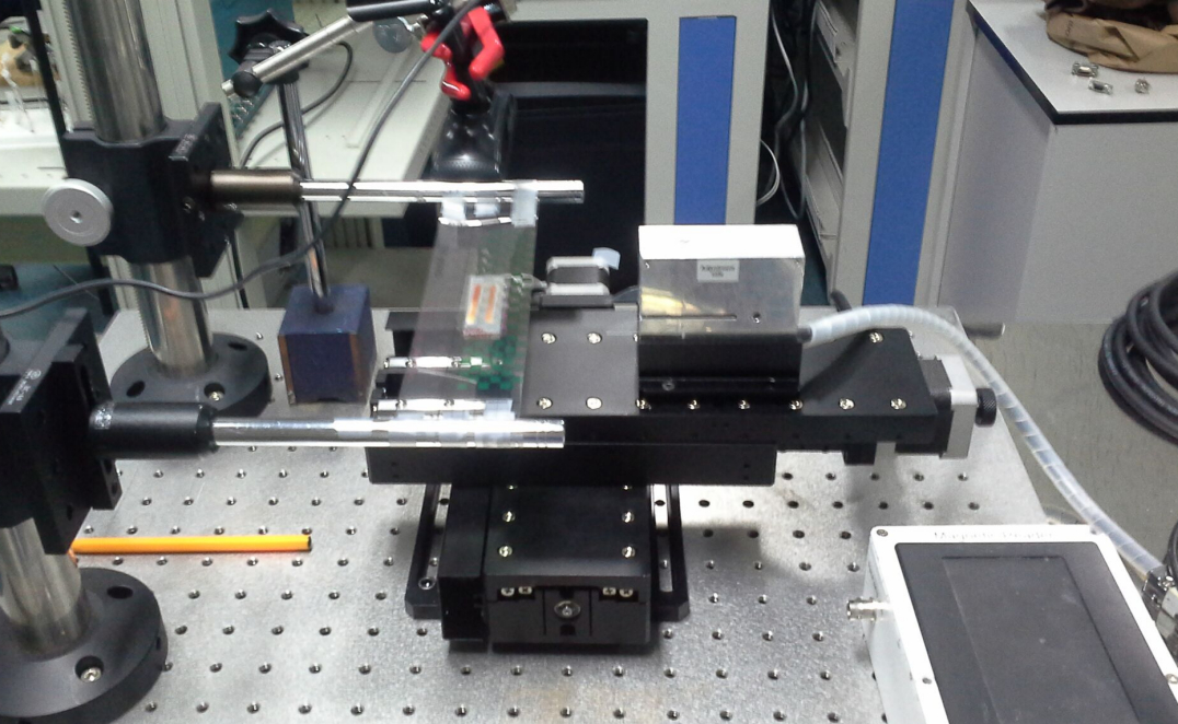
Figure 3. Photo of p-FMMD measurement setup. The sample is affixed with adhesive tape on the plastic carrier moved by the motor stage (left). Then the sample is scanned in the p-FMMD head (right). Please click here to view a larger version of this figure.

6. Perform the scan by pressing the start button. The scans of Figures 5 and 6 cover a 20.0 mm (x axis) × 25.0 mm (y axis) region, i.e., six 25 mm long traces were scanned along the y axis, with 4.0 mm steps in x direction, at a stage speed of 1.0 mm/sec. This amounts to a scanning time of about 2 min.

Figure 4. Graphical User Interface of the scanning software. The scan parameters are entered here. The measurement is started by pressing the red button.

7. Image Processing

1. Convert the raw data to matrix form using a homemade script in python. Log the raw data of the whole scan together with extra values in a 2-column comma-separated values (CSV) format file. The extra column indicates the capturing the corresponding data during the stepping motion. The script segments the raw data column at each change of the extra column value and removes the data segments during stepping motion. It also constructs the resultant matrix by putting the remaining consecutive segments into rows or columns of the matrix and writes the matrix into a CSV format file.
   Note: p-FMMD images of this study are generated using a python script. The pyplot.contour function and the pyplot.imshow function from the matplotlib library for python are cumulatively used for preparation of the contours and the background colors, respectively.

Access restricted. Please log in or start a trial to view this content.

Results

Figure 5a shows the calculated sensitivity distribution of the inner double-differential detection coil as a function of the coordinates x and y in the sample plane. It was calculated in an inverse approach by determining the superposition of the magnetic fields at all points (x, y) in the central plane generated by all four detection coils. In reverse, this determines the detection coil's sensitivity to a magnetic moment at each of...

Access restricted. Please log in or start a trial to view this content.

Discussion

The measurement technique utilizes the nonlinearity of the magnetization curve of the superparamagnetic particles. The two-sided measurement head simultaneously applies two magnetic excitation fields of different frequency to the sample, a low frequency (f₂) component to drive the particles into magnetic saturation and a high frequency (f₁) probe field to measure the nonlinear magnetic response. In particular, both harmonics of the incident fields, m·f_1<...

Access restricted. Please log in or start a trial to view this content.

Materials

Name	Company	Catalog Number	Comments
Magnetic particles "SiMAG Silanol"	Chemicell (http://www.chemicell.com)	1101-5	Aqueous dispersion of magnetic silica particles, Maghemite, dia. 1 µm
Magnetic nanoparticles "fluidMAG-Amine"	Chemicell (http://www.chemicell.com)	4121-5	Aqueous dispersion of magnetic nanoparticles, Magnetite, dia. 50 nm
Microtube 10 µl	Hirschmann Laborgeräte (http://www.hirschmann-laborgeraete.de/?sc_lang=en)		volume 10 µl, outer diameter 400 µm, length 40 mm
Nitrocellulose Membrane Biodyne B	Thermo Scientific (http://www.thermoscientific.com)	77016	Biodyne B Nylon Membrane, 0.45 µm, 8 cm x 12 cm
DDS chip AD9834	Analog Devices (http://www.analog.com)	AD9834	20 mW Power, 2.3 V to 5.5 V, 75 MHz Complete DDS
Operational Amplifier AD829	Analog Devices (http://www.analog.com)	AD829	High Speed, Low Noise Video Op Amp
Analog Multiplier MPY634	Texas Instruments (http://www.ti.com)	MPY634	Wide Bandwidth Precision Analog Multiplier
High-Speed Buffer BUF634	Texas Instruments (http://www.ti.com)	BUF634	250 mA High-Speed Buffer
Operational Amplifier OPA627	Texas Instruments (http://www.ti.com)	OPA627	Precision High-Speed Difet(R) Operational Amplifiers
Operational Amplifier TL072	Texas Instruments (http://www.ti.com)	TL072	Dual Low-Noise JFET-Input General-Purpose Operational Amplifier
Lock-In Amplifier SR830	Stanford Instruments (http://www.thinksrs.com)	SR830	100 kHz DSP lock-in amplifier
XYZ motorized stage	Sciencetown, Incheon, Korea (http://mkmsll.en.ec21.com/)
Cleanroom wiper	Seoul Semitech Co (http://www.seoulsemi.com)	CF-909	dimension 2.0 mm × 18 mm

References

- Tseng, P., Judy, J. W., Di Carlo, D. Magnetic nanoparticle-mediated massively parallel mechanical modulation of single-cell behavior. Nat meth. 9 (11), 1113-1119 (2012).
- Borgert, J., et al. Fundamentals and applications of magnetic particle imaging. J. Cardiovasc. Comput. Tomogr. 6 (3), 149-153 (2012).
- Buzug, T. M., et al. Magnetic particle imaging: introduction to imaging and hardware realization. Z. Med. Phys. 22 (4), 323-334 (2012).
- Kanger, J. S., Subramaniam, V., van Driel, R. Intracellular manipulation of chromatin using magnetic nanoparticles. Chromosome Res. 16 (3), 511-522 (2008).
- Magnetic Nanoparticles: From Fabrication to Clinical Applications. Thanh, N. T. K. , CRC press. Boca Raton. ISBN: 978=1439869321 (2012).
- Saritas, E. U., et al. Magnetic Particle Imaging (MPI) for NMR and MRI researchers. J. Magn. Reson. 229 (4), 116-126 (2012).
- Goodwill, P. W., et al. X-space MPI: magnetic nanoparticles for safe medical imaging. Adv. Mater. 24 (28), 3870-3877 (2012).
- Yim, H., Seo, S., Na, K. MRI Contrast Agent-Based Multifunctional Materials: Diagnosis and Therapy. J Nanomat. 2011 (2011), (2011).
- Gleich, B., Weizenecker, J. Tomographic imaging using the nonlinear response of magnetic particles. Nature. 435 (7046), 1214-1217 (2005).
- Rahmer, J., Weizenecker, J., Gleich, B., Borgert, J. Analysis of a 3-D system function measured for magnetic particle imaging. IEEE Trans. Med. Imaging. 31 (6), 1289-1299 (2012).
- Goodwill, P. W., Conolly, S. M. Multidimensional x-space magnetic particle imaging. IEEE Trans. Med. Imaging. 30 (9), 1581-1590 (2011).
- Goodwill, P. W., Konkle, J. J., Zheng, B., Saritas, E. U., Conolly, S. M. Projection x-space magnetic particle imaging. IEEE Trans. Med. Imaging. 31 (5), 1076-1085 (2012).
- Gräfe, K., et al. An Application Scenario for Single-Sided Magnetic Particle Imaging. Biomed. Tech. 57, Suppl. 1 (2012).
- Krause, H. -J., et al. Magnetic particle detection by frequency mixing for immunoassay applications. J. Magn. Magn. Mater. 311 (1), 436-444 (2007).
- Meyer, M. H. F., et al. Francisella tularensis detection using magnetic labels and a magnetic biosensor based on frequency mixing. J. Magn. Magn. Mater. 311 (1), 259-263 (2007).
- Finas, D., et al. Detection and distribution of superparamagnetic nanoparticles in lymphatic tissue in a breast cancer model for magnetic particle imaging. Biomed. Tech. 57, Suppl. 1 (2012).
- Hong, H., Lim, J., Choi, C. -J., Shin, S. -W., Krause, H. -J. Magnetic particle imaging with a planar frequency mixing magnetic detection scanner. Rev. Sci. Instr. 85 (1), 013705(2014).
- Haegele, J., et al. Toward cardiovascular interventions guided by magnetic particle imaging: First instrument characterization. Magn. Reson. Med. 69 (6), 1761-1767 (2012).
- Haegele, J., et al. Magnetic particle imaging: visualization of instruments for cardiovascular intervention. Radiology. 265 (3), 933-938 (2012).
- Goodwill, P. W., Lu, K., Zheng, B., Conolly, S. M. An x-space magnetic particle imaging scanner. Rev. Sci. Instrum. 83 (3), 033708(2012).
- Lampe, J., et al. Fast reconstruction in magnetic particle imaging. Phys. Med. Biol. 57 (4), 1113-1134 (2012).