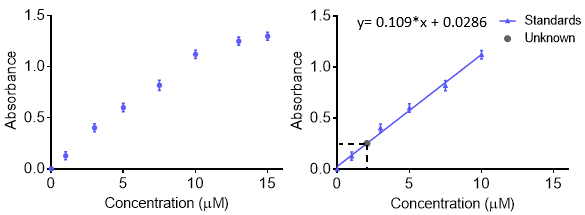
Calibration curves are used to understand the instrumental response to an analyte, and to predict the concentration of analyte in a sample.

A calibration curve is created by first preparing a set of standard solutions with known concentrations of the analyte. The instrument response is measured for each, and plotted vs. concentration of the standard solution. The linear portion of this plot can then be used to predict the concentration of a sample of the analyte, by correlating its response to concentration.

This video will introduce calibration curves and their use, by demonstrating the preparation of a set of standards, followed by the analysis of a sample with unknown concentration.

A set of standard solutions is used to prepare the calibration curve. These solutions consist of a range of concentrations that encompass the approximate concentration of the analyte. 

Standard solutions are often prepared with a serial dilution. A serial dilution is performed by first preparing a stock solution of the analyte. The stock solution is then diluted by a known amount, often one order of magnitude. The new solution is then diluted in the same manner, and so on. This results in a set of solutions with concentrations ranging over several orders of magnitude.

The calibration curve is a plot of instrumental signal vs. concentration. The plot of the standards should be linear, and can be fit with the equation y=mx+b. The non-linear portions of the plot should be discarded, as these concentration ranges are out of the limit of linearity.

The equation of the best-fit line can then be used to determine the concentration of the sample, by using the instrument signal to correlate to concentration. Samples with measurements that lie outside of the linear range of the plot must be diluted, in order to be in the linear range.

The limit of detection of the instrument, or the lowest measurement that can be statistically determined over the noise, can be calculated from the calibration curve as well. A blank sample is measured multiple times. The limit of detection is generally defined as the average blank signal plus 3 times its standard deviation.

Finally, the limit of quantification can also be calculated. The limit of quantification is the lowest amount of analyte that can be accurately quantified. This is calculated as 10 standard deviations above the blank signal.

Now that you've learned the basics of a calibration curve, let's see how to prepare and use one in the laboratory.

First, prepare a concentrated stock solution of the standard. Accurately weigh the standard, and transfer it into a volumetric flask. Add a small amount of solvent, and mix so that the sample dissolves. Then, fill to the line with solvent. It is important to use the same solvent as the sample.

To prepare the standards, pipette the required amount in the volumetric flask. Then fill the flask to the line with solvent, and mix. 

Continue making the standards by pipetting from the stock solution and diluting. For a good calibration curve, at least 5 concentrations are needed.

Now, run samples with the analytical instrument, in this case a UV-Vis spectrophotometer, in order to determine the instrumental response needed for the calibration curve.

Take the measurement of the first standard. Run the standards in random order, in case there are any systematic errors. Measure each standard 3–5x to get an estimate of noise.

Measure the rest of the standards, repeating the measurements for each. Record all data.

Finally, run the sample. Use the same sample matrix and measurement conditions as were used for the standards. Make sure that the sample is within the range of the standards and the limit of the instrument.

To construct the calibration curve, use a computer program to plot the data as signal vs. concentration. Use the standard deviation of the repeated measurements for each data point to make error bars.

Remove portions of the curve that are non-linear, then perform a linear regression and determine the best-fit line. The output should be an equation in the form y = m x + b. An R2-value near 1 denotes a good fit.

This is the calibration curve for blue dye #1, measured at 631 nm. The response is linear between 0 and 15 mM.

Calculate the concentration of the sample using the equation of the best-fit line. The absorbance for the sample was 0.141, and corresponded to a concentration of 6.02 mM.

Now that you've seen how a calibration curve can be used with a UV-Vis spectrophotometer, let's take a look at some other useful applications.

Calibration curves are often used with electrochemistry applications, as the electrode signal must be calibrated to the concentration of ions in the solution. In this example, data were collected for an ion-selective electrode for fluoride.

The concentration data must be plotted on the log scale to obtain a line. This calibration curve can be used to measure the concentration of fluoride in a solution, such as toothpaste or drinking water.

High-performance liquid chromatography, or HPLC, is a separation and analysis technique that is used heavily in analytical chemistry. HPLC separates components of a mixture based on the time required for the molecules to travel the length of the chromatography column. This time varies depending on a range of chemical properties of the molecules.

The elution of the molecules is measured using a detector, resulting in a chromatogram. The peak area can be correlated to concentration using a simple calibration curve of a range of standard solutions, like in this example of popular soda ingredients.

In some cases, where the solution matrix interferes with the measurement of the solute, a classical calibration curve can be inaccurate. In those cases, a modified calibration curve is prepared. For this, a range of standard solution volumes is added to the sample. The signal to concentration plot is created, where the x intercept is equal to the original concentration of the sample solution. For more detail on this technique, please watch the JoVE science education video, "The method of standard addition".

You've just watched JoVE's introduction to the calibration curve. You should now understand where the calibration curve is used, how to create it, and how to use it to calculate concentrations of samples.

As always, thanks for watching!