Watershed Planning within a Quantitative Scenario Analysis Framework

Summary

There is a critical need for tools and methodologies capable of managing aquatic systems in the face of uncertain future conditions. We provide methods for conducting a targeted watershed assessment that enables resource managers to produce landscape-based cumulative effects models for use within a scenario analysis management framework.

Abstract

There is a critical need for tools and methodologies capable of managing aquatic systems within heavily impacted watersheds. Current efforts often fall short as a result of an inability to quantify and predict complex cumulative effects of current and future land use scenarios at relevant spatial scales. The goal of this manuscript is to provide methods for conducting a targeted watershed assessment that enables resource managers to produce landscape-based cumulative effects models for use within a scenario analysis management framework. Sites are first selected for inclusion within the watershed assessment by identifying sites that fall along independent gradients and combinations of known stressors. Field and laboratory techniques are then used to obtain data on the physical, chemical, and biological effects of multiple land use activities. Multiple linear regression analysis is then used to produce landscape-based cumulative effects models for predicting aquatic conditions. Lastly, methods for incorporating cumulative effects models within a scenario analysis framework for guiding management and regulatory decisions (e.g., permitting and mitigation) within actively developing watersheds are discussed and demonstrated for 2 sub-watersheds within the mountaintop mining region of central Appalachia. The watershed assessment and management approach provided herein enables resource managers to facilitate economic and development activity while protecting aquatic resources and producing opportunity for net ecological benefits through targeted remediation.

Introduction

Anthropogenic alteration of natural landscapes is among the greatest current threats to aquatic ecosystems throughout the world¹. In many regions, continued degradation at current rates will result in irreparable damage to aquatic resources, ultimately limiting their capacity to provide invaluable and irreplaceable ecosystem services. Thus, there is a critical need for tools and methodologies capable of managing aquatic systems within developing watersheds^2-3. This is particularly important given that managers are often tasked with conserving aquatic resources in the face of socioeconomic and political pressures to continue development activities.

Management of aquatic systems within actively developing regions requires an ability to predict likely effects of proposed development activities within the context of pre-existing natural and anthropogenic landscape attributes^{3, 4}. A major challenge to aquatic resource management within heavily degraded watersheds is the ability to quantify and manage complex (i.e., additive or interactive) cumulative effects of multiple land use stressors at relevant spatial scales^{2, 5}. Despite current challenges, however, cumulative effects assessments are being incorporated into regulatory guidelines throughout the world^5-6.

Targeted watershed assessments designed to sample the full range of conditions with respect to multiple land use stressors can produce data capable of modeling complex cumulative effects⁷. Moreover, incorporating such models within a scenario analysis framework [predicting ecological changes under a range of realistic or proposed development or watershed management (restoration and mitigation) scenarios] has the potential to greatly improve aquatic resource management within heavily impacted watersheds^{3, 5, 8-9}. Most notably, scenario analysis provides a framework for adding objectivity and transparency to management decisions by incorporating scientific information (ecological relationships and statistical models), regulatory goals, and stakeholder needs into a single decision-making framework^{3, 9}.

We present a methodology for assessing and managing cumulative effects of multiple land use activities within a scenario analysis framework. We first describe how to appropriately target sites for inclusion within the watershed assessment based on known land use stressors. We describe field and laboratory techniques for obtaining data on the ecological effects of multiple land use activities. We briefly describe modeling techniques for producing landscape-based cumulative effects models. Lastly, we discuss how to incorporate cumulative effects models within a scenario analysis framework and demonstrate the utility of this methodology in aiding regulatory decisions (e.g., permitting and restoration) within an intensively mined watershed in southern West Virginia.

Access restricted. Please log in or start a trial to view this content.

Protocol

1. Target Sites for Inclusion in Watershed Assessment

1. Identify the dominant land use activities within the target 8-digit hydrologic unit code (HUC) watershed that are impacting physicochemical and biological condition^{3, 7}.
   Note: This methodology assumes pre-existing knowledge of important stressors within the watershed of interest. However, consulting regulatory agencies or watershed groups familiar with the system can aid in this effort.
2. Select landscape-based measures of dominant land use activities [e.g., 2011 National Land Cover Database (NLCD)] ^{3, 7}.
   1. Consult published literature to help identify the best landscape-based measures for each land use activity¹⁰. Contact natural resource agencies to identify and obtain region-specific landscape datasets that are available for use. However, it may be necessary to create new landscape variables or datasets.
3. Tabulate land cover and use attributes to the 1:24,000 or 1:100,000 national hydrography dataset (NHD) catchments using Geographic Information (GIS) software.
   1. Ensure each 1:24,000 or 1:100,000 catchment has a unique identifier. Use any user-defined numeric or categorical identifier as the unique identifier.
   2. Tabulate vector data (e.g., points or lines) falling within each catchment.
      1. Summarize all vector features within each catchment using the Tabulate Intersection tool within the Statistics toolset of the Analysis toolbox. Select the NHD catchment layer as the Input Zone Feature, the catchment unique identifier as the Zone Field, and the vector dataset of interest as the Input Class Feature.
      2. Join the tabulated landscape attributes to the catchment layer. Right click on the catchments layer in the table of contents and select Joins and Relates from the dropdown menu and Join from the subsequent menu. Select the unique identifier as the field that the join will be based on, the output table from 1.3.2.1 as the table to be joined, and the unique identifier as the field in the table that the join will be based on.
   3. Tabulate raster data using the Tabulate Area tool located within the Zonal toolset of the Spatial Analyst toolbox.
      1. Load the Spatial Analyst extension. Select Extensions from the Customize menu. In the Extensions dialog box, check the box that corresponds to the Spatial Analyst extension.
      2. In the Tabulate Area dialog box, select the NHD catchment shapefile as the input raster or feature zone data, the unique identifier (e.g., FEATUREID) as the zone field, and the land cover dataset (e.g., NLCD) as the input raster or feature class data.
      3. Join the tabulated landscape attributes to the catchment layer following protocols in step 1.3.2.2, with the tabulate area results table as the join table.
4. Accumulate landscape attributes for all NHD catchments.
   1. Download the NHDPlusV2 Catchment Attribute Allocation and Accumulation Tool (CA3TV2) at http://www2.epa.gov/waterdata/nhdplus-tools. Use the accumulation function of CA3TV2 for accumulation of attributes for 1:100,000 NHD catchments ¹¹.
      Note: We used custom written code that accumulates landscape attributes for 1:24,000 scale NHD watersheds¹². Detailed instructions for using CA3TV2 are integrated into the tool and can be accessed via the Help function.
5. Select NHD catchments as study sites based on accumulated landscape attributes.
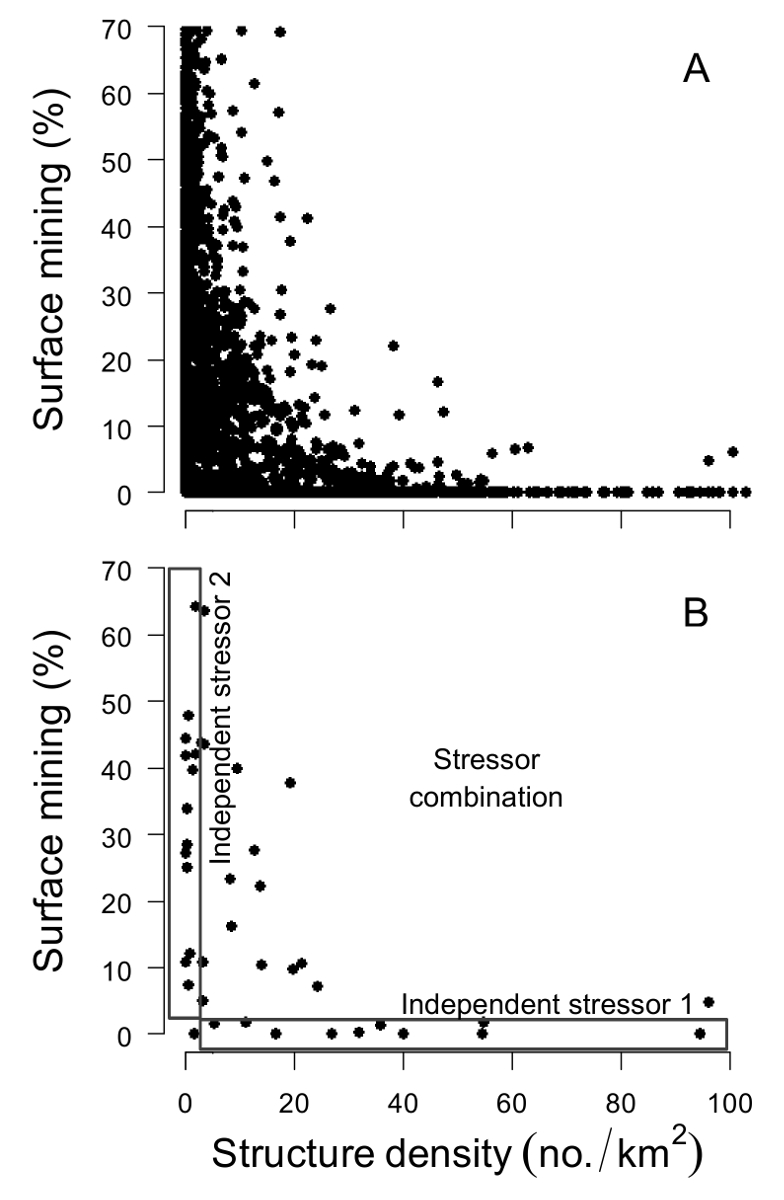
   1. Create a scatter plot of all NHD catchments with respect to accumulated values of major land use activities (Figure 1A).
   2. Select study sites (approximately 40 sites per 8-digit HUC watershed) to represent the full range of influence from dominant land use activities found within the target watershed (Figure 1B). Select sites within independent stressor gradients (i.e., influenced by a single land use activity) and stressor combinations (i.e., influenced by multiple land use activities) (Figure 1B).
   3. Ensure that study sites are spatially distributed throughout the target watershed and independent of one another with respect to downstream drainage. Ensure that sites falling within each individual and combined stressor gradient also have similar average basin areas.

Figure 1. Hypothetical scatter plot of NHD catchments with respect to influence from 2 land use activities. Magnitude of influence of 2 land use activities across all NHD catchments within the hypothetical watershed (n=4,229) (A). Selected study sites (n=40) that represent the full range of observed conditions within the watershed with respect to independent and combined stressor gradients (B). Please click here to view a larger version of this figure.

2. Field Protocols for Collection of Physicochemical and Biological Data

Note: All data for each site should be collected during the same site visit at normal base flow conditions. Protocols presented herein represent standard operating procedures for the West Virginia Department of Environmental Protection (WVDEP)¹³. It may be more appropriate to use state or federally recognized procedures for the specific watershed being assessed.

1. Delineate the sampling reach for each site as 40× active channel width (ACW), with maximum and minimum lengths of 150 and 300 m^{3, 7}.
2. Sample water quality attributes from locations with moving water that are characteristic of the entire sampling site (e.g., not directly influenced by tributary or drainage pipe inputs).
   1. Obtain instantaneous measures of dissolved oxygen, specific conductivity, temperature, and pH using handheld sensors. Calibrate sensors prior to each sampling event following manufacturer instructions.
   2. Rinse filtration equipment with deionized water prior to water sample collection.
   3. Filter 250 ml of water (mixed cellulose ester membrane filter, 0.45 µm pore size) for analysis of dissolved metals. Fix to a pH<2 to ensure metals remain dissolved in solution.
      Note: The correct volume of acid can be added to the water sample following sample collection. Alternatively, the correct volume can be added to the bottle prior to the sampling event. The volume required to fix to a pH<2 is dependent upon acid strength.
      1. For the study described here, collect a single filtered sample from each site and fix with nitric acid for determination of dissolved Al, Ca, Fe, Mg, Mn, Na, Zn, K, Ba, Cd, Cr, Ni, and Se^{3, 7}.
         Note: Selection of analytes should be guided by watershed-specific land use activities.
   4. Collect 250 ml unfiltered sample(s) by completely submerging the sample bottle in the water column. Gently squeeze the bottle to expunge any remaining air and simultaneously place the cap on the sample bottle. Fix the sample(s) to a pH <2 if necessary (e.g., prevent biological activity from affecting nutrients).
      1. For the study described here, collect two unfiltered samples from each site. Fix the first with sulfuric acid for determination of NO₂ and NO₃ and total P. Do not fix the second unfiltered sample and use it to determine total and bicarbonate alkalinity, Cl, SO₄, and total dissolved solids^{3, 7}.
         Note: Selection of analytes should be guided by watershed-specific land use activities.
   5. Obtain a field blank for each fixative used during each sampling event. Obtain field blanks by following all protocols for sample collection (i.e., rinsing, filtering, fixing) using deionized water as the final sample.
      Note: Field blanks are used to identify contamination in sample collection and analysis.
   6. Store all water samples at 4 °C until all analyses are completed. Ensure all analytes are measured within their specified holding time¹⁴.
3. Measure discharge at each sample site.
   1. Divide the wetted stream width into equal-sized increments.
   2. Measure depth and average current velocity at the mid-point of each section.
      1. Using a depth gauge rod, measure depth as the distance from the stream bed to the water's surface.
      2. Using a current meter, measure water velocity at 60% water depth.
   3. Calculate discharge as the sum of the product of velocity, depth, and width across all sections.
4. Sample the macroinvertebrate community at each site.
   1. Obtain kick samples (net dimensions 335 × 508 mm² with 500-µm mesh) from 4 separate representative riffles distributed throughout the entire length of the sampling reach.
      1. At each kick location, place the kick net perpendicular to stream flow and disturb a 0.50 × 0.50 m² (i.e., 0.25 m²) area of the stream bed immediately upstream. Ensure all organisms and debris flow downstream into the kick net.
      2. Combine organisms and debris from the 4 kick samples into a single composite sample (representing 1.00 m² of the stream bed) and immediately preserve with 95% ethanol.
5. Measure physical habitat quality and complexity throughout the stream reach.
   1. Take measurements of water depth, hydraulic channel-unit type, sediment class, and distance to fish cover object at evenly spaced points along the thalweg (portion of the stream through which the main or most rapid flow occurs). Take measurements every 1 ACW for streams <5 m wide and every 0.5 ACW for streams >5 m wide¹⁵.
      1. Classify the channel unit within which each thalweg location is located (e.g., riffle, run, pool, or glide)¹⁶.
      2. Using a depth gauge rod, measure depth as the distance from the stream bed to the water's surface.
      3. Randomly identify a piece of sediment and determine its Wentworth size classification (silt, sand, gravel, cobble, boulder)¹⁷.
      4. Estimate the distance from each thalweg point to the nearest cover object.
         Note: Fish cover is defined as any structure in the active channel capable of concealing a 20.32 cm (8 in) fish¹⁸.
   2. Count all pieces of large woody debris within the active channel.
   3. Estimate habitat quality with US Environmental Protection Agency (EPA) rapid visual habitat assessments (RVHA) protocols¹⁹.
6. Obtain duplicate measurements and samples from a randomly selected 10% of study sites. Duplicate measures are used to estimate sampling and laboratory analysis precision.

3. Laboratory Protocols for Physicochemical and Biological Data

Note: Describing laboratory protocols for quantifying water chemistry attributes is outside the scope of this manuscript. However, the current study used standard chemical methods for water and wastes¹⁴.

1. Subsample organisms contained within each macroinvertebrate sample (collected using protocols in section 2.4) to obtain a representative subsample of the macroinvertebrate community at each site.
   1. Place the entire composite macroinvertebrate sample into a 100 in² gridded sorting (measuring 5 × 20 in²). Randomly assign each 1 in² grid a number from 1 to 100.
   2. Use a stereo microscope to count and identify all organisms within randomly selected 1 in² grids until the total number of sorted individuals is 200 ± 20%. Identify organisms to genus using macroinvertebrate keys, such as those published by Merritt and Cummins²⁰.
   3. Compile genus-level abundance data into community metrics [e.g., total richness and % Ephemeroptera, Plecoptera, and Trichoptera (EPT)] for use as response variables in statistical models and subsequent scenario analysis^{3, 7}.

4. Statistical and Scenario Analyses

1. Construct generalized linear models for predicting in-stream physical, chemical, and biological conditions from landscape-based indicators of dominant land use activities.
   Note: Protocols and analyses were performed in the R language and environment for statistical computing (version 3.2.1)²¹.
   1. Test for normality using Shapiro-Wilk [shaprio.test() function in R package stats²¹] tests and transform variables to meet assumptions of parametric analyses and linearize relationships.
   2. Fit initial maximal models specifying 2-way interactions among all land use predictors [glm() function in R package stats²¹].
   3. Apply a backward deletion to identify the minimum adequate model^{3, 7, 22}.
      1. Identify the least significant (i.e., explains the least amount of variation) variable in the maximal model [summary() function in R package stats²¹] and fit a new model with this variable excluded [glm () function in R package stats²¹].
      2. Continue removing variables until all remaining predictors are significantly different from 0 and explanatory power does not differ significantly from the maximal model for each response variable using analysis of deviance tables and likelihood ratio tests [lrtest() function in R package lmtest²³].
2. Predict current conditions.
   1. Use final models to predict physicochemical and biological condition given current landscape characteristics within all un-sampled NHD catchments throughout the target watershed [predict() function in R package stats²¹].
   2. Visualize predictions in GIS software.
      1. Join predictions to NHD catchments. Right click on the catchments layer in the table of contents and select Joins and Relates from the dropdown menu and Join from the subsequent menu. Select the unique identifier as the field that the join will be based on, the predictions file as the table to be joined, and the unique identifier as the field in the table that the join will be based on
      2. Right click on the catchments layer and select Properties. In the Layer Properties dialog box, click on the Symbology tab and select Quantities. Select the predicted value of interest as the Value field and click Apply.
         Note: Range values can be manually changed to match recognized ecological criteria using the Classify button.
3. Conduct scenario analyses to compare predicted changes in aquatic conditions under various land use scenarios.
   1. Update the current landscape dataset to simulate plausible future development or mitigation scenarios. For the study described here, manually update accumulated landscape values for the catchment of interest within the attribute table (e.g., change 10 acres of forested to mining land cover).
      1. Select the catchment of interest using the Select by Attribute function located within the Selection drop down menu. In the Select by Attribute dialog box, choose the NHD catchments as the Layer. Double click on the unique identifier attribute, select =, and then type the identifier for the catchment of interest in the equation box.
      2. Open the NHD catchment attribute table by right clicking the catchments layer in the table of contents and selecting Open Attribute Table from the drop down menu. Choose to show only selected catchments.
      3. With only selected catchments showing, right click on the column of interest and select Field Calculator and input the new simulated value. Note: Multiple catchments can be altered to simulate multiple spatially explicit development or management activities occurring across large spatial scales.
         Note: Alternatively, original vector and raster datasets can be updated by digitizing new features or altering and removing original features to simulate new land use activity or management of a pre-existing land use impact²⁴. This can be accomplished using the Editor Toolbar.
   2. Re-allocate and re-accumulate landscape attributes for all NHD catchments using protocols presented in steps 1.3-1.4.
   3. Predict physicochemical and biological condition as a function of the updated landscape dataset [predict() function in R package stats²¹].
   4. Visualize predicted conditions under alternative land use scenarios using protocols presented in step 4.2.2.

Access restricted. Please log in or start a trial to view this content.

Results

Forty 1:24,000 NHD catchments were selected as study sites within the Coal River, West Virginia (Figure 2). Study sites were selected to span a range influence from surface mining (% land area²⁴), residential development [structure density (no./km²)], and underground mining [national pollution discharge elimination system (NPDES) permit density (no./km²)] such that each major land use activity occurred both in isolation and in combination ...

Access restricted. Please log in or start a trial to view this content.

Discussion

We provide a framework for assessing and managing cumulative effects of multiple land use activities in heavily impacted watersheds. The approach described herein addresses previously identified limitations associated with managing aquatic systems in heavily impacted watersheds^5-6. Most notably, the targeted watershed assessment design (i.e., sampling along individual and combined stressor axes) produces data that are well suited for quantifying complex cumulative effects at relevant spatial scales (<...

Access restricted. Please log in or start a trial to view this content.

Materials

Name	Company	Catalog Number	Comments
Slack Invert Sampling Kit	Wildco	3-425-N56
HDPE Square Jars	US Plastic Corp	66188	32 oz; for storing fixed, composite invertebrate samples
Ethyl Alcohol 190 Proof	PHARMCO-AAPER	111000190	For fixing and storing invertebrate samples
5 in. by 20 in. Macroinvertebrate sub-samplilng grid	N/A	N/A	This item cannot be purchased and must be made in house
Stereomicroscope Stemi 2000 with stand C LED	ZEISS	000000-1106-133	For macroinvertebrate sorting and identification
Thermo Scientific Nalgene Reusable Filter Holders with Receiver	Fisher Scientific	09-740-23A
Immobilon-NC Transfer Membrane	Millipore	HATF04700	Triton-free, mixed cellulose exters, 0.45 μm, 47 mm, disc
Actron Vacuum Pump Brake Bleeder Kit	Advanced Auto Parts	CP7835
Nitric Acid Solution	HACH	254049	1:1, 500 ml
Oblong NDPE Wide Mouth Bottles	Thomas Scientific	1229Z38	250 ml; for collection of water samples
650 Multi-parameter display, standard memory	Fondriest Environmental	650-01
600XL Sonde with temperature/conductivity sensor	Fondriest Environmental	065862
pH calibration buffer pack	Fondriest Environmental	603824	2 pints each of pH 4, 7, & 10
conductivity standard	Fondriest Environmental	065270	1 quart, 1,000 µS
Flo-Mate 2000	TTT Environmental	2000-11
Keson English/Metric Open Reel Fiberglass Tape	Forestry Suppliers	40025	300'/100 m
ArcGIS 10.3.1	ESRI

References

- Allan, J. D. Landscapes and riverscapes: the influence of land use on stream ecosystems. Annu. Rev. Ecol. Evol. Syst. 35, 257-284 (2004).
- Merovich, G. T., Petty, J. T., Strager, M. P., Fulton, J. B. Hierarchical classification of stream condition: a house-neighborhood framework for establishing conservartion priorities in complex riverscapes. Freshwater Science. 32, 874-891 (2013).
- Merriam, E. R., Petty, J. T., Strager, M. P., Maxwell, A. E., Ziemkiewicz, P. F. Scenario analysis predicts context-dependent stream response to land use change in a heavily mined central Appalachian watershed. Freshwater Science. 32, 1246-1259 (2013).
- Petty, J. T., Fulton, J. B., Strager, M. P., Merovich, G. T., Stiles, J. M., Ziemkiewicz, P. F. Landscape indicators and thresholds of stream ecological impairment in an intensively mined Appalachian watershed. J. N. Am. Benthol. Soc. 29, 1292-1309 (2010).
- Seitz, N. E., Westbrook, C. J., Noble, B. F. Bringing science into river systems cumulative effects assessment practice. Environ. Impact Asses. 31, 172-179 (2011).
- Duinker, P. N., Greig, L. A. The importance of cumulative effects assessment in Canada: ailments and ideas for redeployment. Environ. Manage. 37, 153-161 (2006).
- Merriam, E. R., Petty, J. T., Strager, M. P., Maxwell, A. E., Ziemkiewicz, P. F. Landscape-based cumulative effects models for predicting stream response to mountaintop mining in multistressor Appalachian watersheds. Freshwater Science. 34, 1006-1019 (2015).
- Duinker, P. N., Greig, L. A. Scenario analysis in environmental impact assessment: improving explorations of the future. Environ. Impact Asses. 27, 206-219 (2007).
- Kepner, W. G., Ramsey, M. M., Brown, E. S., Jarchow, M. E., Dickinson, K. J. M., Mark, A. F. Hydrologic futures: using scenario analysis to evaluate impacts of forecasted land use change on hydrologic services. Ecosphere. 3, 1-25 (2012).
- Gergel, S. E., Turner, M. G., Miller, J. R., Melack, J. M., Stanley, E. H. Landscape indicators of human impacts to riverine systems. Aquat. Sci. 64, 118-128 (2002).
- McKay, L., Bondelid, T., Dewald, T., Johnston, J., Moore, R., Rea, A. NHDPlus Version 2: User Guide. , (2012).
- Strager, M. P., Petty, J. T., Strager, J. M., Barker-Fulton, J. A spatially explicit framework for quantifying downstream hydrologic conditions. J. Environ. Manag. 90, 1854-1861 (2009).
- WVDEP (Virginia Department of Environmental Protection). Standard operating proceedures. , West Virgina Department of Environmental Protection. Charleston, West Virginia. (2009).
- EPA-60014-79-020. USEPA. Methods for chemical analysis of water and wastes. , Environmental Monitoring Systems Support Laboratory, Office of Research and Development, US Environmental Protection Agency. Cincinnati, Ohio. (1983).
- Merriam, E. R., Petty, J. T., Merovich, G. T., Fulton, J. B., Strager, M. P. Additive effects of mining and residential development on stream conditions in a central Appalachian watershed. J. N. Am. Benthol. Soc. 30, 399-418 (2011).
- Bisson, P. A., Nielsen, J. L., Palmason, R. A., Grove, L. E. A system of naming habitat types in streams, with examples of habitat utilization by salmonids during low streamflow. Acquisition and utilization of aquatic habitat inventory information. Proceedings of a symposium held 28-30 October, 1981. Armentrout, N. D. , Western Division of the American Fisheries Society. Bathesda, Maryland. 62-73 (1982).
- Wentworth, C. K. A scale of grade and class terms for clastic sediments. J. Geol. 30, 377-392 (1922).
- Petty, J. T., Freund, J., Lamothe, P., Mazik, P. Quantifying instream habitat in the upper Shavers Fork basin at multiple spatial scales. Proceedings of the Annual Conference of the Southeastern Association of Fisheries and Wildlife Agencies. 55, 81-94 (2001).
- Barbour, M. T., Gerritsen, J., Snyder, B. D., Stribling, J. B. EPA/841-B-99-022. Rapid bioassessment protocols for use in streams and wadeable rivers: periphyton, benthic macroinvertebrates, and fish. 2nd edition. , US Environmental Protection Agency. Washington, DC. (1999).
- An introduction to the aquatic insects of North America. 4th edition. Merritt, R. W., Cummins, K. W. , Kendall/Hunt Publishing Co. Dubuque, Iowa. (2008).
- A language and environment for statistical computing. , R Foundation for Statistical Computing. Vienna, Austria, http://www.R-project.org. Available from: http://www.R-project.org (2014).
- Crawley, M. J. Statistics: an introduction using R. , Wiley and Sons. Chichester, UK. (2005).
- Zeileis, A., Hothorn, T. Diagnostic Checking in Regression Relationships. R News. 2, 7-10 (2002).
- Maxwell, A. E., Strager, M. P., Yuill, C., Petty, J. T., Merriam, E. R., Mazzarella, C. Disturbance mapping and landscape modeling of mountaintop mining using ArcGIS. Proceedings of the ESRI International User Conference. , San Diego, California. (2011).
- Gerritsen, J., Burton, J., Barbour, M. T. A stream condition index for West Virginia wadeable streams. , Tetra Tech, Inc. Owings Mills, Maryland. (2000).
- Pond, G. J., Passmore, M. E., Borsuk, F. A., Reynolds, L., Rose, C. J. Downstream effects of mountaintop coal mining: comparing biological conditions using family- and genus-level macroinvertebrate bioassessment tools. J. N. Am. Benthol. Soc. 27, 717-737 (2008).
- Luo, Y., et al. Ecological forecasting and data assimilation in a data-rich era. Ecol. Appl. 21, 1429-1442 (2011).
- Petty, J. T., Strager, M. P., Merriam, E. R., Ziemkiewicz, P. F. Scenario analysis and the Watershed Futures Planner: predicting future aquatic condiditons in an intensively mined Appalachian watershed. Environmental Considerations in Energy Productions. Craynon, J. R. , Society for Mining, Metallurgy, and Exploration. Englewood, CO. 5-19 (2013).
- Daraio, J. A., Bales, J. D. Effects of land use and climate change on stream temperature I: daily flow and stream temperature projections. J. Am. Water Resour. As. 50, 1155-1176 (2014).
- Mantyka-Pringle, C. S., Martin, T. G., Moffatt, D. B., Linke, S., Rhodes, J. R. Understanding and predicting the combined effects of climate change and land-use change on freshwater macroinvertebrates and fish. J. Appl. Ecol. 51, 572-581 (2014).
- Piggott, J. J., Townsend, C. R., Matthaei, C. D. Climate warming and agricultural stressors interact to determine stream macroinvertebrate community dynamics. Glob. Change Biol. 21, 1897-1906 (2015).
- Elith, J., Leathwick, J. R., Hastie, T. A working guide to boosted regression trees. J. Anim. Ecol. 77, 802-813 (2008).
- Mattson, K. M., Angermeier, P. L. Integrating human impacts and ecological integrity into a risk-based protocol for conservation planning. Environ. Manage. 39, 125-138 (2007).
- EPA 841-B-11-002. USEPA. Identifying and protecting healthy watersheds. Concepts, assessments, and management approaches. (US, U. S. E. P. A. , US Environment Protection Agency, Office of Water, Office of Wetlands, Oceans, and Watersheds. Washington, DC. (2012).
- Merriam, E. R., Petty, J. T., Strager, M. P., Maxwell, A. E., Ziemkiewicz, P. F. Complex contaminant mixtures in multi-stressor Appalachian riverscapes. Environ. Toxicol. Chem. , (2015).