溶存有機物生物地球化学を理解します<em&gt;その場で</em&gt;ストリーム生態系における栄養操作を

要約

Dissolved organic matter provides an important source of energy and nutrients to stream ecosystems. Here we demonstrate a field-based method to manipulate the ambient pool of dissolved organic matter in situ through easily replicable nutrient pulses.

要約

Dissolved organic matter (DOM) is a highly diverse mixture of molecules providing one of the largest sources of energy and nutrients to stream ecosystems. Yet the in situ study of DOM is difficult as the molecular complexity of the DOM pool cannot be easily reproduced for experimental purposes. Nutrient additions to streams however, have been shown to repeatedly alter the in situ and ambient DOM pool. Here we demonstrate an easily replicable field-based method for manipulating the ambient pool of DOM at the ecosystem scale. During nutrient pulse experiments changes in the concentration of both dissolved organic carbon and dissolved organic nitrogen can be examined across a wide-range of nutrient concentrations. This method allows researchers to examine the controls on the DOM pool and make inferences regarding the role and function that certain fractions of the DOM pool play within ecosystems. We advocate the use of this method as a technique to help develop a deeper understanding of DOM biogeochemistry and how it interacts with nutrients. With further development this method may help elucidate the dynamics of DOM in other ecosystems.

概要

溶存有機物（DOM）は、生態系を淡水する重要なエネルギー及び栄養源を提供し、0.7μmのフィルターを通過する有機物として定義されます。水界生態系の中では、DOMは、光の減衰と金属錯体形成に影響を与えることができます。 DOMは、種々の官能基を有する有機化合物、並びに窒素（N）とリン（P）などの必須栄養素の非常に多様かつ不均一な混合物です。用語「DOM」はそのC、NおよびP成分を含むプール全体を説明しているが、その濃度は、溶存有機炭素（DOC）として測定されます。 DOMプールの固有の分子の複雑さは、しかし、その研究への挑戦を作成します。例えば、このような溶存有機態窒素（DON）と溶存有機リン（DOP）などの有機栄養素からなる総DOMプールの割合を測定する直接的な方法はありません。代わりに、有機栄養素の濃度の差によって決定されなければなりません（ 例えば[DON] = [総溶存窒素] - [溶存無機窒素]）。

ストリームに現実的なDOMの修正を追加することは、周囲のDOMプールの多様性のために困難です。以前の研究では、単一の炭素源（ 例えば、グルコース、尿素^1）を追加しました または落葉浸出液²のような特定のソースは、フィールド中の濃度を操作することができます。しかし、これらのソースは、周囲のDOMプールの特に代表的なものではありません。その後の実験のために周囲のDOMを絞り込むか、集中しようとすると、処理中の特定の画分（ 例えば 、高度に不安定な部品）の損失を含む困難に細工されています。その結果、我々は、現在、直接周囲DOMプールを操作する任意の方法を持たないように、周囲のDOMプールのコントロールを理解することは困難です。しかし、DOMの生物地球化学は、 例えば 、NIT（一般的な環境で見つかった栄養素にリンクされているので、レート[NO ₃ ^- ] ^3）、私たちは生態系をストリーミングし、これらの操作にDOMプールの応答を測定する他の溶質を追加することができます。 DOMプールは、我々はDOMは環境条件の変動にどのように応答するかをより深い洞察を得るために願って実験的に課せられた栄養広範囲の濃度にどのように応答するかを調べることによって。

一般的にストリームの生物地球化学に使用される1つの方法は、栄養添加方法です。栄養添加実験は、伝統的に取り込み速度または添加溶質^4,5,6,7-の運命を理解するために使用されてきました。栄養添加物は、複数年⁸にわたって日スケール^4、または長期的な操作に時間⁶に短期的であることができます。生物地球化学反応を介して追加された栄養素をトレースする^-栄養添加物はまた、同位体標識された栄養素（ 例えば^、15 N-NO _3）を含むことができます。しかし、同位体ベースの研究は、多くの場合、EXPEですnsiveと同位体で標識された栄養素を保持することができる複数の底生区画の挑戦的な分析（ 例えば消化）が必要です。最近の実験はその場生物地球化学的反応でリアルタイムに検討することにより、新しい方法を明らかにし、そのようなDOM ^9,10-などの非添加し、周囲の溶質上のコントロールを解明する短期的な栄養パルスの有用性を明らかにしました。ここでは説明し、非常に多様なDOMプールでCとNと特異的にコントロールの結合された生物地球化学を理解することを目的とした短期的な栄養パルスを実施するための鍵の方法論の手順を示しています。この簡単に再現性のある方法は、実験的なストリームリーチに栄養パルスを追加し、操作溶質と関心の応答変数（ 例えば DOC、DON、DOP）の両方の濃度の変化を測定することを含みます。直接その場で栄養濃度を操作することによって、我々は間接的にDOMを変更することができます栄養濃度¹⁰のダイナミックレンジ全体でどのようにDOMの濃度変化をプールし、検討します。

プロトコル

1. Identifying and Characterizing the Ideal Experimental Stream Reach

1. Ensure that experimental stream reaches are long enough to promote complete mixing of solutes¹¹ and long enough where biological uptake can occur. Reach lengths can vary among streams and experiments. In small first-order headwater streams, reach length may vary from 20-150 m (or longer if the system requires it) depending on discharge and other physical properties of the stream.
   1. Exclude large pools from experimental reaches, as they retard the downstream movement of solutes, minimal flow sections, and tributaries that dilute the added solution. Times of low discharge may require shortening the reach length while higher discharge may require a longer reach.
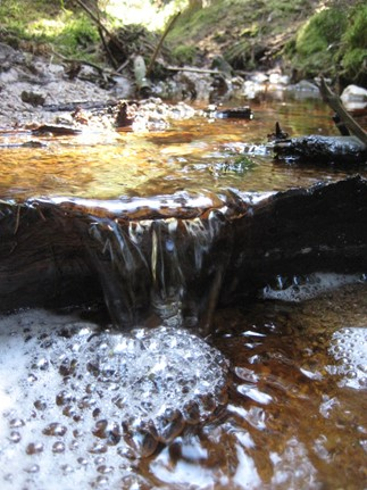
   2. Identify a location at the top of the experimental stream reach above a riffle to facilitate mixing of the added solutes. This will be the addition site. At the bottom of the experimental stream reach, identify a location where flow is constricted and representative of about 90% of the total flow (Figure 1). This will be the sample collection site.

Figure 1: Example of Downstream Sampling Site. An ideal sampling site is where the majority of flow is constricted and easily accessible without disturbance of the stream channel and benthos. Here a fallen piece of wood debris has created this sampling point in a small first-order headwater stream. Please click here to view a larger version of this figure.

2. Obtain discharge measurement and background nutrient concentrations of the solutes of interest prior to experiments in order to calculate the mass of solutes needed for the manipulations. Please see calculations in step 2.2.1.
   1. Obtain background concentration data for the target solute of manipulation (e.g. NO₃^-) and chloride (Cl^-) which is often used as the conservative tracer. Use the conservative tracer in the context of these experiments, to track changes in conductivity, which indicate the arrival of the nutrient pulse at the sampling station and the rate in which the pulse is passing through. Conductivity, or specific conductance, is a surrogate for in-situ changes in concentration of the conservative tracer.
   2. Characterize the physio-chemical properties of the experimental reach by collecting ancillary data such as reach width and depth, temperature, pH and dissolved oxygen.
      1. Perform measurements that cannot be made with the use of an environmental probe (e.g. width and depth), the day before or immediately after the experiment in order to minimize any benthic or chemical disturbance within the stream channel. Divide the experimental reach in equidistant transects (e.g. every 10 m) where width and at least 3 depth measurements can be assessed (e.g. right bank, thalweg, and left bank). These data are valuable to connect the physical properties of a stream to biogeochemical measurements and if the researchers are also interested in calculating nutrient uptake kinetics and parameters⁶.

2. Preparation for Experiment

1. Determine the mass (kg) of solute required for manipulation using the outlined equations below.
   Note: The example below applies to a nitrate-based experiment with NO₃^- in the form of sodium nitrate (NaNO₃) and assumes a targeted increase of 3x above background (equations are based on those of Kilpatrick and Cobb¹²). In this example the following assumptions have been made with respect to background conditions: discharge = 10 L/sec; [Cl] = 10 mg/L; [NO₃^-] = 50 µg N/L. Due to variation among experiments, adjust required input data.
   1. Calculate the Targeted increase (Equation 1):
      Targeted [NO₃- μg N/L] increase = expected background [NO₃- μg N/L] * targeted increase
      150 μg N/L = 50 μg N/L * 3
   2. Calculate the total atomic mass flux (Equation 2):
      Total atomic mass flux (NO₃- μg N) = 30 min * 60 sec * Q(L/sec) * targeted [NO₃- μg N/L] increase
      Where 30 minutes is the assumed duration of solute peak¹² and Q is discharge
      2 700 000 μg N = 30 min * 60 sec * 10 L/s * 150 μg N/L
   3. Calculate the total molecular mass flux (Equation 3):
      Total molecular mass flux (NO₃- μg N) = total atomic mass flux (NO₃- μg N)/atomic mass (14) * molecular weight (85)
      Where atomic mass refers to N and molecular weight refers to NaNO₃.
      16,392,857.14 μg N = 2,700,000 μg N/(14 * 85) 
   4. Calculate the mass to add (Equation 4):
      Mass to add (g) = total molecular mass flux (NO₃- μg N)/1,000,000 g/μg
      16.39 g NaNO₃ = 16,392,857.14 μg N/1,000,000 g/μg
      Note: Follow the above calculations for any other solutes including the conservative tracer (e.g. sodium chloride). Make sure to adjust the atomic and molecular masses for the solute of interest.
2. Prepare all solutes one day prior to field experiments. Weigh out enough solutes to raise the ambient concentration of both the biological tracer and the conservative tracer three times (or desired amount) above background. It is important that the quantity of added solutes causes a measureable change above background concentration that is sufficient to create a wide dynamic range in added nutrient concentration.
   1. Weigh solutes using analytical scales and subsequently store in clean acid-washed high-density polyethylene bottles with appropriate labels. Examples of biological tracers include: NO₃^-: sodium nitrate (NaNO₃); NH₄⁺: ammonium chloride (NH₄Cl); PO₄^-3: potassium phosphate (K₂HPO₄). However, the choice of biological tracer will be a function of the biogeochemical question being asked. Options for conservative tracers include sodium chloride (NaCl) and sodium bromide (NaBr).
3. Collect remaining materials: field book, labeling tape and pen, field measuring tape, cooler, conductivity meter, ~ 20 L bucket and large stirring rod (e.g. beer paddle, rebar, large stick), approximately 50 clean and acid-washed 125 ml high-density polyethylene bottles. Label the 125 ml bottles #1-50.
   Note: Less than 50 samples can be taken per experiment and background samples are included in the 50 total bottles.
4. Optional: Depending on the numbers of field personnel, perform sample filtering on-site (see section #5). If this option is chosen, bring 50 clean, pre-labeled and acid-washed 60 ml high-density polyethylene bottles into the field. Label the 60 ml bottles #1-50 to match the 125 ml collection bottles.

3. Day of Set Up

1. Deploy the field conductivity meter at the collection site. Place the instrument upstream (approximately 0.5-1.0 m) of where samples will be taken so sample collection does not interfere with instrument readings. The meter will remain in place throughout the experiment. A field conductivity meter is best as it provides real-time conductivity readings, which are required to determine the sampling rate (see step 5.2) and filtration and analysis order (steps 5.3 and 6.1).
2. Collect 125 ml background samples in triplicate at the addition site and at the collection site of the experimental reach prior to the addition of the solution. These data will be used to verify day-of ambient concentration and to determine variation in solute concentration along the stream reach. These data are also valuable to connect ambient stream chemistry (e.g. DOC: NO₃^- ratios¹³) to the biogeochemical measurements of interest.
3. Record the time and conductivity of background samples collected.
4. Record the background conductivity of stream prior to addition of solutions.

4. Adding Solutes

1. Pour all reagents (16.39 g NaNO₃ and 1483 g NaCl) into a large container (e.g. 20 L bucket) and add enough stream water to completely dissolve the solutes. Rinse reagent vessels thrice with additional stream water and pour rinse into solution container. Keep track of amount of water added.
   1. For example, use a 500 ml bottle to pour stream water into the container. Stir solution until all reagents have been completely dissolved.
2. Collect 60 ml aliquot of the addition solution. Keep this highly concentrated sample separate (e.g. zip-lock bag) from all other samples to minimize cross contamination. Such samples are important if calculating nutrient uptake kinetics⁶ is an additional goal of the research project as these samples can be used to determine the exact mass of solutes added.
3. Pour solution into addition site. Do this by pouring the solution in a smooth and quick motion to minimize travel lag time and splashing that could reduce the amount of reagents added. Rinse the container and the stir stick three times in the stream immediately after the addition to guarantee all reagents have been added to the stream.
   1. Record the time the solution was added: hr:min:sec.
   2. Record the masses of tracers added (e.g. NaNO₃ and NaCl).
   3. After the solution has been added, do not disturb the stream. Make sure that all travel along the stream occurs on the banks to ensure that the stream benthos and the solution itself are not disturbed.

5. Field Sampling

1. Order sampling bottles in ascending order while waiting for solution to arrive to the sampling location. Travel time will be a function of discharge and reach length and can be determined ahead of time (one-day prior) either with a NaCl-only injection or rhodamine dye (which can be used to establish travel time¹⁴).
   Note: If working on a DON-themed project, avoid using rhodamine dye as it is a type of DON and will therefore alter the ambient DON pool if any remains in the study reach.

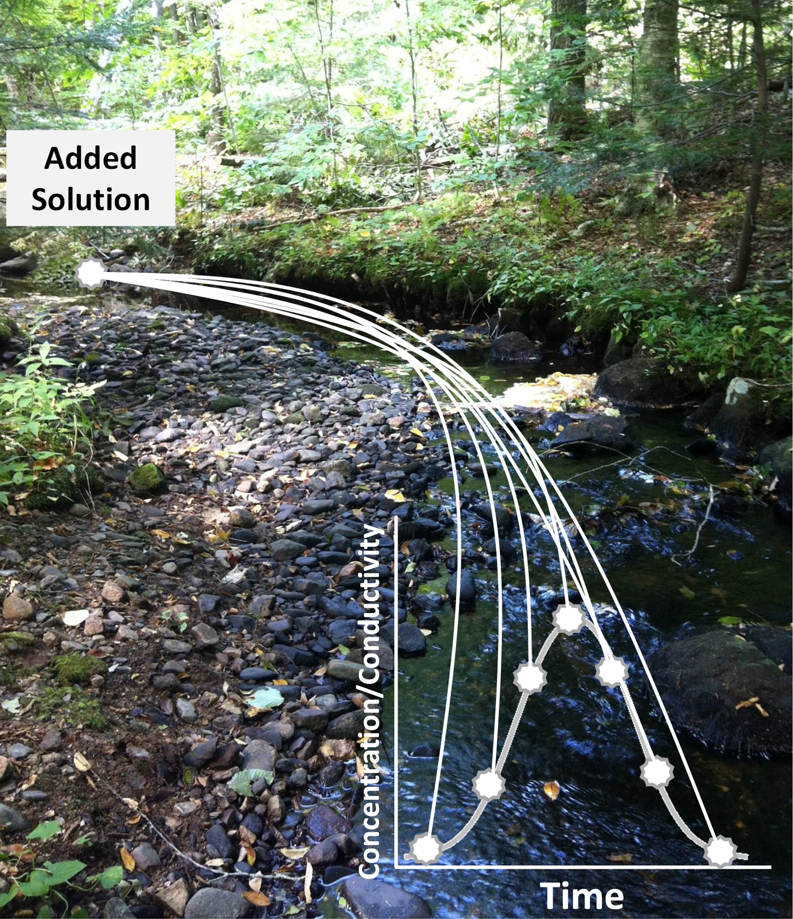
Figure 2: Example Schematic of Solute Breakthrough Curve (BTC). A BTC represents changes in solute concentration over time and can be used to explain the transit and biogeochemical cycling of a tracer in a stream. Grab samples should be taken across the BTC with a frequency that gives equal representation to both the ascending and descending limbs of the BTC. Please click here to view a larger version of this figure.

2. Sample Collection
   Note: The over-arching objective of sample collection, is to adequately represent changes in solute concentration along both the rising and falling limbs of the break through curve (BTC) (Figure 2).
   1. Upon arrival of the solution (detected via an increase in conductivity), collect samples in 125 ml bottles throughout the BTC by holding a 125 ml bottle into the main flow of water at the sampling point. Quickly rinse the bottle with stream water and discard rinse downstream and then take sample. Cap sample and place into cooler.
   2. Record the time (hr:min:sec) and conductivity of each sample taken along the BTC into a field book (Table 1).
   3. Collect samples based on time (e.g. 1 min intervals) or based on the rate at which conductivity changes. For example, if conductivity is changing quickly, sample every 30-60 sec until changes in conductivity slow, at which time samples can be taken every 5-10 min. For intervals based on conductivity, take samples every 15-30 units depending on the rate at which conductivity is changing.
   4. Sample until conductivity returns to background or within 5 µS/cm of background conditions. Intervals of sample collection can be adjusted during the experiment as long as the BTC is well represented in the grab samples.

Bottle #	Specific Conductance	Time	Notes
1		hr:min:sec	e.g. background (downstream)
2			e.g. background (downstream)
3
4
5			e.g. sample at peak conductance
.
.
.
Highest Bottle #

Table 1PField book: Example Page from Lab Book and Required Information

3. Sample Filtering
   Note: Filtering of samples can occur either in the field or upon returning to the laboratory.
   1. Filter samples from the rising limb in order of ascending specific conductivity until the peak in specific conductivity. Wait for the experiment to be over and filter samples from the falling limb in ascending order of specific conductivity (i.e. start with the last sample and work backwards toward peak specific conductivity).
      Note: This order of samples minimizes cross contamination between samples and allows for the same filter, syringe, and filter holder to be used as long as the filter, syringe and filter holder are appropriately rinsed in between each sample (see steps 5.3.2-5.3.4).
   2. Remove plunger from a 60 ml syringe and then close stop-cock. Pour ~10 ml of sample into syringe and return plunger to syringe. Shake syringe so that sample rinses internal walls of syringe. Attached syringe to filter-holder and open stop-cock. Push sample through filter-holder and discard rinse.
   3. Remove plunger and close stop-cock. Pour ~30 ml of sample into syringe and return plunger to syringe. Open stock-cock and expel ~10 ml through filter-holder and into 60 ml sampling bottle. Cap the bottle, swirl with filtrate and discard. Repeat this step for a total of 3 rinses. This will ensure any impurities have been removed from the 60 ml sample bottle and that the walls are coated with sample.
   4. Remove plunger and close stop-cock. Pour ~60 ml of sample into syringe and return plunger to syringe. Push the sample through the filter holder and into the 60 ml sample bottle. Fill bottles up to the shoulder to prevent cracking of bottles when frozen. Cap bottle and place into cooler.
   5. Repeat steps 5.3.2-5.3.4 for all remaining samples. Change filter between rising and falling limb samples to minimize contamination.
   6. Transport samples back to the laboratory on the same day and on ice.

6. Preparation for Laboratory Analysis

1. If filtering of samples is to occur in the laboratory, follow protocol as outlined in section 5.3.1. Filter samples from both the ascending and descending limbs of the BTC in order of increasing conductivity. Change the filter between rising limb and falling limb samples.
2. Freeze filtered samples at -20 °C until analysis.
3. Ensure that analytical facilities are equipped to handle highly concentrated samples.
   Note: Some laboratories are not equipped to run highly concentrated samples and thus care should be taken. Incorporate prepared standards that capture that higher end of expected solute concentrations. High concentration standards will help to ensure a standard curve that captures the expected range of manipulated solute concentrations.
4. Analyze samples from low to high conductivity on all analytical instruments. Ordering samples from low to high specific conductance prevents contamination of low salt/nutrient samples by high salt/nutrient samples. This means samples from the rising and falling limbs will be mixed with respect to sequence.
   1. Analyze samples for total dissolved organic carbon, total dissolved nitrogen, nitrate and ammonium, although the exact combination of solute analysis will be a function of the research question (see Wymore et al.¹⁰ for example).

7. Data Analysis

1. Analyze the data using simple linear regression. The independent variable is the concentrations of the added nutrient and the dependent variable is DOM concentration either as DOC or DON. Each point on the figure represents one grab sample from the breakthrough curve and that sample's nutrient and DOC/DON concentration.

結果

Figure 3: Example Results from Nitrate (NO₃^-) Additions with Dissolved Organic Nitrogen (DON) as the Response Variable. Analyses are linear regressions. Asterisks represent statistical significance at α = 0.05. Note the dynamic range in NO₃^- concentration that was achieved with the nutrient pulse method. Different pane...

ディスカッション

The objective of the nutrient pulse method, as presented here, is to characterize and quantify the response of the highly diverse pool of ambient stream water DOM across a dynamic range of an added inorganic nutrient. If the added solute sufficiently increases the concentration of the reactive solute, a large inferential space can be created to understand how the biogeochemical cycling of DOM is linked to nutrient concentrations. This nutrient pulse approach is ideal as it involves none of the machinery associated with p...

資料

Name	Company	Catalog Number	Comments
Sodium Nitrate	Any	Any
Sodium Chloride	Any	Any	Store purchased table salt can be used as well, however, it does contain trace levels of impurities
Whatman GFF glass-fiber filters	Any	Any
BD Filtering Syringe	Any	Any
EMD Millipore Swinnex Filter Holders	Any	Any
Syringe stop-cock	Any	Any
YSI Multi-parameter probe	Yellow Springs International	556-01
Wide mouth HDPE 125 ml bottles	Any	Any
60 ml HDPE bottles	Any	Any
20 L bucket	Any	Any
Field measuring tape	Any	Any
Lab labeling tape	Any	Any
Stir stick	Any	Any
Cooler	Any	Any
Sharpie pen	Any	Any
Field notebook	Any	Any
Tweezers	Any	Any
Zip-lock bags	Any	Any