A Workflow for Lipid Nanoparticle (LNP) Formulation Optimization using Designed Mixture-Process Experiments and Self-Validated Ensemble Models (SVEM)

Podsumowanie

This protocol provides an approach to formulation optimization over mixture, continuous, and categorical study factors that minimizes subjective choices in the experimental design construction. For the analysis phase, an effective and easy-to-use modeling fitting procedure is employed.

Streszczenie

We present a Quality by Design (QbD) styled approach for optimizing lipid nanoparticle (LNP) formulations, aiming to offer scientists an accessible workflow. The inherent restriction in these studies, where the molar ratios of ionizable, helper, and PEG lipids must add up to 100%, requires specialized design and analysis methods to accommodate this mixture constraint. Focusing on lipid and process factors that are commonly used in LNP design optimization, we provide steps that avoid many of the difficulties that traditionally arise in the design and analysis of mixture-process experiments by employing space-filling designs and utilizing the recently developed statistical framework of self-validated ensemble models (SVEM). In addition to producing candidate optimal formulations, the workflow also builds graphical summaries of the fitted statistical models that simplify the interpretation of the results. The newly identified candidate formulations are assessed with confirmation runs and optionally can be conducted in the context of a more comprehensive second-phase study.

Wprowadzenie

Lipid nanoparticle (LNP) formulations for in vivo gene delivery systems generally involve four constituent lipids from the categories of ionizable, helper, and PEG lipids^1,2,3. Whether these lipids are being studied alone or simultaneously with other non-mixture factors, experiments for these formulations require "mixture" designs because - given a candidate formulation - increasing or decreasing the ratio of any one of the lipids necessarily leads to a corresponding decrease or increase in the sum of the ratios of the other three lipids.

For illustration, it is supposed that we are optimizing an LNP formulation that currently uses a set recipe that will be treated as the benchmark. The goal is to maximize the potency of the LNP while secondarily aiming to minimize the average particle size. The study factors that are varied in the experiment are the molar ratios of the four constituent lipids (ionizable, cholesterol, DOPE, PEG), the N:P ratio, the flow rate, and the ionizable lipid type. The ionizable and helper lipids (including cholesterol) are allowed to vary over a wider range of molar ratio, 10-60%, than PEG, which will be varied from 1-5% in this illustration. The benchmark formulation recipe and the ranges of the other factors and their rounding granularity are specified in Supplementary File 1. For this example, the scientists are able to perform 23 runs (unique batches of particles) in a single day and would like to use that as their sample size if it meets the minimum requirements. Simulated results for this experiment are provided in Supplementary File 2 and Supplementary File 3.

Rampado and Peer⁴ have published a recent review paper on the topic of designed experiments for the optimization of nanoparticle-based drug delivery systems. Kauffman et al.⁵ considered LNP optimization studies using fractional factorial and definitive screening designs⁶; however, these types of designs cannot accommodate a mixture constraint without resorting to the use of inefficient "slack variables"⁷ and are not typically used when mixture factors are present^7,8. Instead, "optimal designs" capable of incorporating a mixture constraint are traditionally used for mixture-process experiments⁹. These designs target a user-specified function of the study factors and are only optimal (in one of a number of possible senses) if this function captures the true relationship between the study factors and responses. Note that there is a distinction in the text between "optimal designs" and "optimal formulation candidates", with the latter referring to the best formulations identified by a statistical model. Optimal designs come with three main disadvantages for mixture-process experiments. First, if the scientist fails to anticipate an interaction of the study factors when specifying the target model, then the resulting model will be biased and can produce inferior candidate formulations. Second, optimal designs place most of the runs on the exterior boundary of the factor space. In LNP studies, this can lead to a large number of lost runs if the particles do not form correctly at any extremes of the lipid or process settings. Third, scientists often prefer to have experimental runs on the interior of the factor space to gain a model-independent sense of the response surface and to observe the process directly in previously unexplored regions of the factor space.

An alternative design principle is to target an approximate uniform coverage of the (mixture-constrained) factor space with a space-filling design¹⁰. These designs sacrifice some experimental efficiency relative to optimal designs⁹ (assuming the entire factor space leads to valid formulations) but present several benefits in a trade-off that are useful in this application. The space-filling design does not make any a priori assumptions about the structure of the response surface; this gives it the flexibility to capture unanticipated relationships between the study factors. This also streamlines the design generation because it does not require making decisions about which regression terms to add or remove as the desired run size is adjusted. When some design points (recipes) lead to failed formulations, space-filling designs make it possible to model the failure boundary over the study factors while also supporting statistical models for the study responses over the successful factor combinations. Finally, the interior coverage of the factor space allows for model-independent graphical exploration of the response surface.

To visualize the mixture factor subspace of a mixture-process experiment, specialized triangular "ternary plots" are used. Figure 1 motivates this usage: in the cube of points where three ingredients are each allowed to range from 0 to 1, the points that satisfy a constraint that the sum of the ingredients equals 1 are highlighted in red. The mixture constraint on the three ingredients reduces the feasible factor space to a triangle. In LNP applications with four mixture ingredients, we produce six different ternary plots to represent the factor space by plotting two lipids at a time against an "Others" axis that represents the sum of the other lipids.

Figure 1: Triangular factor regions. In the space-filling plot within the cube, the small grey dots represent formulations that are inconsistent with the mixture constraint. The larger red points lie on a triangle inscribed within the cube and represent formulations for which the mixture constraint is satisfied. Please click here to view a larger version of this figure.

In addition to the lipid mixture factors, there are often one or more continuous process factors such as N:P ratio, buffer concentration, or flow rate. Categorical factors may be present, such as ionizable lipid type, helper lipid type, or buffer type. The goal is to find a formulation (a mixture of lipids and settings for process factors) that maximizes some measure of potency and/or improves physiochemical characteristics such as minimizing particle size and PDI (polydispersity index), maximizing percent encapsulation, and minimizing side effects - such as body weight loss - in in vivo studies. Even when starting from a reasonable benchmark recipe, there may be interest in re-optimizing given a change in the genetic payload or when considering changes in the process factors or lipid types.

Cornell⁷ provides a definitive text on the statistical aspects of mixture and mixture-process experiments, with Myers et al.⁹ providing an excellent summary of the most relevant mixture design and analysis topics for optimization. However, these works can overload scientists with statistical details and with specialized terminology. Modern software for the design and analysis of experiments provides a robust solution that will sufficiently support most LNP optimization problems without having to appeal to the relevant theory. While more complicated or high-priority studies will still benefit from collaboration with a statistician and may employ optimal rather than space-filling designs, our goal is to improve the comfort level of scientists and to encourage optimization of LNP formulations without appealing to inefficient one-factor-at-a-time (OFAT) testing¹¹ or simply settling for the first formulation that satisfies specifications.

In this article, a workflow is presented that utilizes statistical software to optimize a generic LNP formulation problem, addressing design and analysis issues in the order that they will be encountered. In fact, the method will work for general optimization problems and is not restricted to LNPs. Along the way, several common questions that arise are addressed and recommendations are provided that are grounded in experience and in simulation results¹². The recently developed framework of self-validated ensemble models (SVEM)¹³ has greatly improved the otherwise fragile approach to analyzing results from mixture-process experiments, and we use this approach to provide a simplified strategy for formulation optimization. While the workflow is constructed in a general manner that could be followed using other software packages, JMP 17 Pro is unique in offering SVEM along with the graphical summary tools that we have found to be necessary to simplify the otherwise arcane analysis of mixture-process experiments. As a result, JMP-specific instructions are also provided in the protocol.

SVEM employs the same linear regression model foundation as the traditional approach, but it allows us to avoid tedious modifications that are required to fit a "full model" of candidate effects by using either a forward selection or a penalized selection (Lasso) base approach. Additionally, SVEM provides an improved "reduced model" fit that minimizes the potential for incorporating noise (process plus analytical variance) that appears in the data. It works by averaging the predicted models resulting from repeatedly reweighting the relative importance of each run in the model^{13,14,15,16,17,18}. SVEM provides a framework for modeling mixture-process experiments that is both easier to implement than traditional single-shot regression and yields better quality optimal formulation candidates^12,13. The mathematical details of SVEM are beyond the scope of this paper and even a cursory summary beyond the relevant literature review would distract from its main advantage in this application: it allows a simple, robust, and accurate click-to-run procedure for practitioners.

The presented workflow is consistent with the Quality by Design (QbD)¹⁹ approach to pharmaceutical development²⁰. The result of the study will be an understanding of the functional relationship that links the material attributes and process parameters to critical quality attributes (CQAs)²¹. Daniel et al.²² discuss using a QbD framework specifically for RNA platform production: our workflow could be used as a tool within this framework.

Protokół

The experiment described in the Representative Results section was carried out in accordance with the Guide for the Care and Use of Laboratory Animals and the procedures were performed following guidelines established by our Institutional Animal Care and Use Committee (IACUC). 6-8 week old female Balb/C mice were commercially obtained. Animals received ad libitum standard chow and water and were housed under standard conditions with 12 hour light/dark cycles, at a temperature of 65-75 °F (~18-23 °C) with 40-60% humidity.

1. Recording the study purpose, responses, and factors

NOTE: Throughout this protocol, JMP 17 Pro is used for designing and analyzing the experiment. Equivalent software can be used following similar steps. For examples and further instructions for all the steps performed in Section 1, please refer to Supplementary File 1.

1. Summarize the purpose of the experiment in a date-stamped document.
2. List the primary responses (CQAs) that will be measured during the experiment.
3. List any secondary responses (e.g., downstream restrictions on physiochemical properties) that might be measured.
4. List process parameters that may be related to the responses, including those that are most relevant to the purpose of the study.
5. If the study will run over multiple days include a Day categorical "blocking" factor.
   NOTE: This balances factor settings across days to prevent day-level shifts in the process mean from being confounded with the study factors.
6. Select the factors to be varied and those to be held constant during the study.
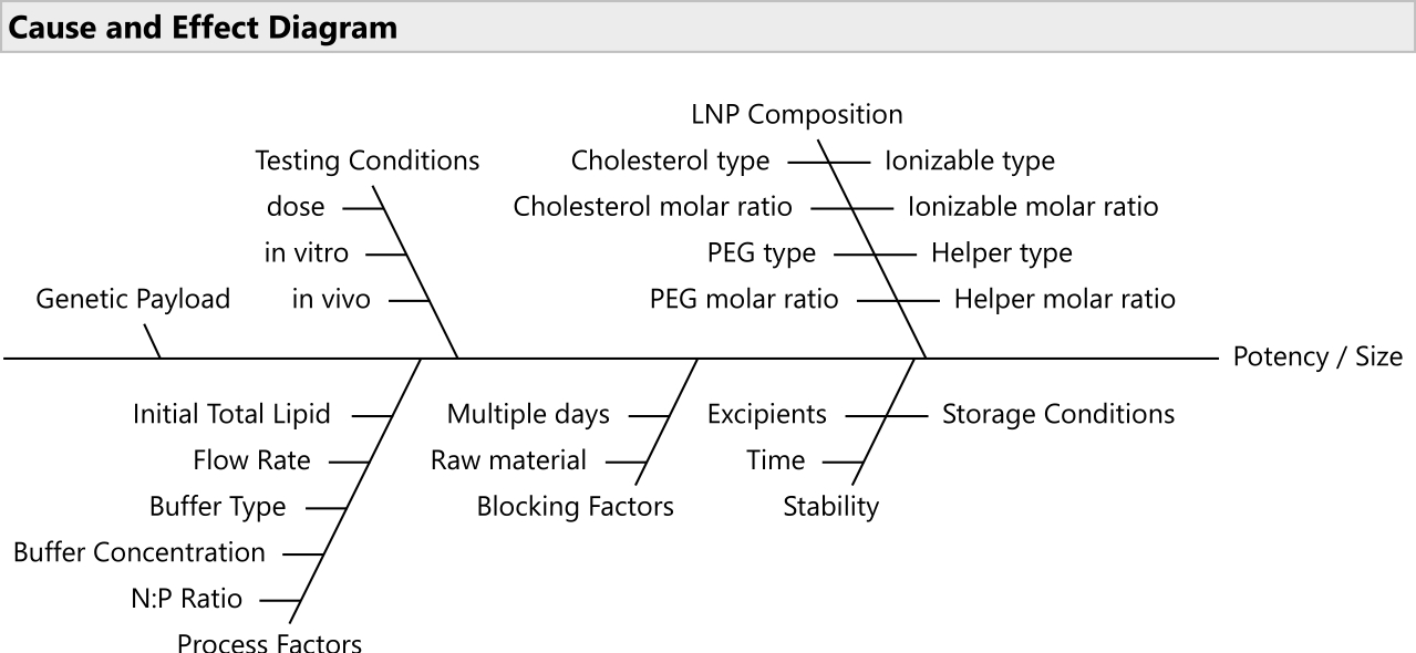
   NOTE: Use risk prioritization tools like failure mode effects analyses²⁰ for selecting the most relevant subset of factors (Figure 2). Usually, all lipids should be allowed to vary; although in some budget-constrained cases, it is reasonable to lock PEG at a fixed ratio.
7. Establish the ranges for the varying factors and the relevant decimal precision for each.
8. Decide the study design size (the number of unique batches of particles) using the minimum and maximum heuristics. Manually-included control benchmark runs do not count toward the run size recommended by the heuristics.
   NOTE: The following heuristics assume the responses are continuous. The minimum heuristic assumes that it will be possible to perform a follow-up study, if needed, in addition to performing confirmation runs for candidate optimal formulations. If it will only be feasible to perform confirmation runs, then it is better to budget for the number of runs obtained from the maximum heuristic. For binary primary responses, seek help from a statistician to determine the appropriate number of runs.
   1. Minimum heuristic: Allocate three runs per mixture factor, two per continuous process factor, and one per level of each categorical factor.
      NOTE: For a study with four lipid factors, two continuous, and one three-way categorical process variable, this leads to a suggestion of (3 x 4) + (2 x 2) + 3=19 space-filling runs. Add additional runs if some are likely to fail due to formulation or measurement issues.
   2. Maximum heuristic: Launch the software for building optimal designs and input the required parameters for a second order (including main effects, two-way interactions between all effects, and quadratic effects for continuous process factors). Calculate the minimum run size as per the software's algorithm. Add 1 to the result obtained from the software to define the maximum heuristic.
      NOTE: Refer to Supplementary File 1 for detailed instructions on performing these steps. A sample case with four lipid factors, two continuous and one three-way categorical process variable, leads to a recommended run size of 34 (33 from software recommendation + 1). Any runs beyond this would likely be better used for confirmation or follow-up studies.

Figure 2: Cause and effect diagram. The diagram shows common factors in an LNP formulation optimization problem. Please click here to view a larger version of this figure.

2. Creation of the design table with a space-filling design

1. Open JMP and navigate the menu bar to DOE > Special Purpose > Space Filling Design.
2. Enter the study responses (see Supplementary File 1).
3. Optional: Add columns for additional responses, indicating if each is to be maximized, minimized, or targeted by clicking Add Response.
   NOTE: These settings can be modified later and do not affect the design. Likewise, additional columns for additional responses may be added after creating the design table.
4. Enter the study factors and the corresponding ranges. Use the Mixture button to add mixture factors, the Continuous button to add continuous factors, or the Categorical button to add categorical factors.
   NOTE: This example study uses the factors and ranges illustrated in Figure 3, which include the Ionizable molar ratio (ranging between 0.1 and 0.6), the Helper molar ratio (also between 0.1 and 0.6), the Cholesterol molar ratio (between 0.1 and 0.6), the PEG molar ratio (from 0.01 to 0.05), and the Ionizable Lipid Type (which can be H101, H102, or H103).
5. Input the predetermined number of runs for the design into the Number of Runs field.
6. Optional: Increase the Average Cluster Size from the default of 50 to 2000 via the red triangle menu next to the Space Filling Design header and in the Advanced Options submenu.
   NOTE: This is a setting for the space-filling algorithm that can lead to slightly better design construction at the cost of additional computational time.
7. Generate the space-filling design table for the chosen factors and run size. Click Fast Flexible Filling, then click Make Table.
   NOTE: The first two runs from an example design are shown in Figure 4.
8. Add a Notes column to the table for annotating any manually created runs. Double-click the first empty column header to add a column, and then double-click the new column header to edit the name.
9. If applicable, manually incorporate benchmark control runs into the design table. Include a replicate for one of the control benchmarks. Mark the benchmark name in the Notes column and color-code the benchmark replicate rows for easy graph identification.
   1. Add a new row by double-clicking the first empty row header and input the benchmark factor settings. Duplicate this row to create a replicate of the benchmark. Highlight both rows and navigate to Rows > Colors to assign a color for graphing purposes.
      NOTE: The replicate provides a model-independent estimate of the process plus analytical variance and will provide additional graphical insight.
10. If any benchmark control runs exceed the range of the study factors, denote this in the "Notes" column for future exclusion from analysis.
11. Round the mixture factors to the appropriate granularity. To do so,
    1. Highlight the column headers for the mixture factors, right-click one of the column headers, and navigate to New Formula Column > Transform > Round…, input the correct rounding interval, and click OK.
    2. Make sure no rows are selected by clicking the bottom triangle at the intersection of row and column headers.
    3. Copy the values from the newly created rounded columns (Ctrl + C) and paste (Ctrl + V) into the original mixture columns. Finally, delete the temporary rounded value columns.
12. After rounding the lipid ratios, verify their sum equals 100% by selecting the column headers for the mixture factors, right-clicking one, and going to New Formula Column > Combine > Sum. If any row's sum does not equal 1, manually adjust one of the mixture factors, ensuring the factor setting stays within the factor range. Delete the sum column after adjustments are done.
13. Follow the same procedure used for rounding the mixture factors to round the process factors to their respective granularity.
14. Format the lipid columns to display as percentages with the desired number of decimals: select the column headers, right-click, and choose Standardize Attributes.... In the next window, set Format to Percent and adjust the number of decimals as needed.
15. If manual runs are added such as benchmarks, re-randomize the table row order: add a new column with random values (Right-click the last column header and select New Formula Column > Random > Random Normal). Sort this column in ascending order by right-clicking on its column header, and then delete the column.
16. Optional: add a Run ID column. Populate this with the current date, experiment name, and row number from the table.
    NOTE: See (Figure 5) for an example.
17. Generate ternary plots to visualize the design points over the lipid factors (Figure 6). Also, examine the run distribution over the process factors (Figure 7): select Graph > Ternary Plot. Select only the mixture factors for X, Plotting.
18. To examine the distribution over the process factors, select Analyze > Distribution and enter the process factors for Y, Columns.
    NOTE: The formulation scientist should confirm the feasibility of all runs. If infeasible runs exist, restart the design considering the newly discovered constraints.

Figure 3: Study factors and ranges. Screenshots of settings within experimental software are useful for reproducing the study setup. Please click here to view a larger version of this figure.

Figure 4: Initial output for a space-filling design. Showing the first two rows of the table, settings need to be rounded to the desired precision while also making sure that the lipid amounts sum to 1. The benchmark was added to the table manually. Please click here to view a larger version of this figure.

Figure 5: Formatted study table. The factor levels have been rounded and formatted and a Run ID column has been added. Please click here to view a larger version of this figure.

Figure 6: Design points on a ternary plot. The 23 formulations are shown as a function of the corresponding Ionizable, Helper and "Others" (Cholesterol+PEG) ratios. The green point in the center represents the benchmark 33:33:33:1 molar ratio of Ionizable (H101):Cholesterol:Helper (DOPE):PEG. Please click here to view a larger version of this figure.

Figure 7: Distribution of non-mixture process factors in the experiment. The histograms show how the experimental runs are spaced across Ionizable Lipid Type, N:P ratio, and Flow Rate. Please click here to view a larger version of this figure.

3. Running the experiment

1. Run the experiment in the order provided by the design table. Record the readouts in the columns built into the experimental table.
2. If multiple assays are performed for the same response on an identical formulation batch, calculate an average for these results within each batch. Add a column for each assay measurement to the table.
   1. To obtain an average, select all related columns, right-click on one of the selected column headers, and choose New Formula Column > Combine > Average. Use this Average column for future response analysis.
      NOTE: Without starting the recipe anew, repeated assay measurements only capture assay variance and do not constitute independent replicates.
3. Document any occurrence of formulation precipitation or in vivo tolerability issues (such as severe body weight loss or death) with binary (0/1) indicators in a new column for each type of issue.

4. Analyzing the experimental results

1. Plot the readings and examine the distributions of the responses: open Graph > Graph Builder and drag each response into the Y area for individual plots. Repeat this for all responses.
2. Examine the relative distance between the color-coded replicate runs, if one was included. This allows for the understanding of the total (process and analytic) variation at the benchmark compared to the variability due to changes in the factor settings across the entire factor space (Figure 8).
3. Determine if the raw response should be modeled or if a transformation should be used instead. For responses that are restricted to being positive but are unbounded above (e.g., potency), fit both a normal distribution and a lognormal distribution to the experimental results. If the lognormal distribution fits better with a lower AICc (corrected Akaike's Information Criterion), then take a log transformation of that response.
   1. Navigate to Analyze > Distribution and select the response for Y, Columns. In the resulting distribution report, click the red triangle next to the response name and choose Continuous Fit > Fit Normal and Continuous Fit > Fit Lognormal from the drop-down menu. In the subsequent Compare Distributions report, check the AICc values to ascertain which distribution fits the response better.
   2. To perform a log transform, right-click the response column header and select New Formula Column > Log > Log. When a model is built and a prediction column on the log scale is saved, transform the response back to the original scale by selecting New Formula Column > Log > Exp.
   3. For proportion responses bounded between 0 and 1, compare the fit of a normal and beta distribution. If the beta distribution has a lower AICc, perform a logit transform. In the Distribution report for the response, choose Continuous Fit > Fit Normal and Continuous Fit > Fit Beta.
      1. For the logit transform, right-click the response column header in the data table, and select New Formula Column > Specialty > Logit. Post model-building, save the prediction column. To revert to the original scale, use New Formula Column > Specialty > Logistic.
         NOTE: The regression-based SVEM analysis is robust to departures from normality in the response distribution. However, these transformations can lead to easier interpretation of the results and to an improved fit of the models.
4. Graph the runs on a ternary plot. Color the points according to the responses (or the transformed responses if a transformation was applied): open Graph > Ternary Plot. Select only the mixture factors for X, Plotting. Right-click on any of the resulting graphs, select Row Legend and then select the (transformed) response column.
   NOTE: Coloring the points according to responses gives a model-independent visual perspective of behavior in relation to mixture factors.
5. Delete the Model script generated by the Space-Filling Design. 
6. Build an independent model for each response as a function of the study factors, repeating the following steps for each response.
   NOTE: In the case of a secondary binary response (e.g., formulation failure or mouse death), model this response as well. Change the target distribution setting from Normal to Binomial.
7. Construct a "full" model comprising all candidate effects. This model should include the main effects of each factor, two- and three-way interactions, quadratic and partial cubic terms in the process factors, and Scheffé cubic terms for the mixture factors^23,24.
   NOTE: Use the same set of candidate effects for each response. The SVEM model selection technique will independently refine the models for each response, potentially resulting in unique reduced models for each one. Figure 9 illustrates some of these candidate effects. The following sub-steps detail this process.
   1. Select Analyze > Fit Model.
   2. Ensure blocking factors (e.g., Day) are not allowed to interact with other study factors. Select any blocking factors and click Add. Do not include these factors in any of the subsequent sub-steps.
      NOTE: Blocking factors are important to account for in the model but blocking factors should not be allowed to interact with other study factors. The main purpose of blocking factors is to help control the experiment's variability and improve the sensitivity of the experiment.
   3. Highlight all of the study factors. Modify the Degree field value to 3 (it is set to 2 by default). Click on Factorial to Degree.
      NOTE: This action includes main effects as well as two- and three-way interactions in the model.
   4. Select only the non-mixture factors in the selection window. Click Macros > Partial Cubic.
      NOTE: This action introduces quadratic effects for the continuous process factors and their interaction with other non-mixture factors in the model.
   5. Choose only the mixture factors from the selection list. Click Macros > Scheffe Cubic. Deactivate the default No Intercept option (refer to Figure 9).
      NOTE: Including an intercept in the model is an essential step when using Lasso methods and is also helpful in the forward selection context. The traditional default setting No Intercept is usually in place because fitting an intercept simultaneously with all the mixture main effects, without modifications such as the SVEM approach, is not feasible with the regular least squares regression procedure¹².
   6. Specify the response column: highlight the response column and click Y.
   7. Change the Personality setting to Generalized Regression. Keep Distribution set to Normal.
   8. Save this model setup to the data table for use with additional responses by clicking on the red triangle menu next to Model Specification and selecting Save to Data Table.
8. Apply the SVEM forward selection method to fit the reduced model, without mandatory inclusion of the mixture factor main effects, and store the prediction formula column in the data table.
   1. From the Fit Model dialog, click Run.
   2. For the Estimation Method, select SVEM Forward Selection.
   3. Expand the Advanced Controls > Force Terms menus and deselect the boxes associated with the mixture's main effects. Only the Intercept term box should remain checked. Figure 10 displays the default setup where the main effects are forced. For this step, these boxes need to be unchecked to allow the model to include or exclude these effects based on the forward selection procedure.
   4. Click Go to run the SVEM Forward Selection procedure.
9. Plot the actual responses by the predicted responses from the SVEM model to verify a reasonable predictive ability. (Figure 11). Click the red triangle next to SVEM Forward Selection and select Diagnostic Plots > Plot Actual by Predicted.
10. Click the red triangle next to SVEM Forward Selection and select Save Columns > Save Prediction Formula to create a new column containing the prediction formula in the data table.
11. Optional: Repeat the above steps using SVEM Lasso as the Estimation Method to determine if a different optimal recipe is suggested after performing the subsequent steps. If so, run both recipes as confirmation runs (discussed in Section 5) to see which performs best in practice¹².
12. Repeat the model-building steps for each response.
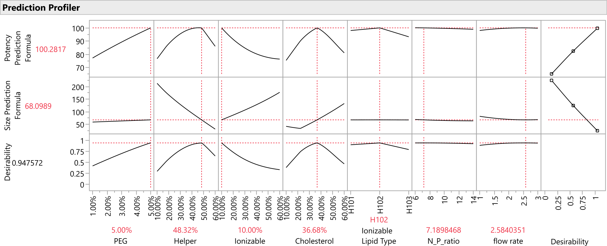
13. Once prediction columns for all responses are saved to the data table, graph the response traces for all predicted response columns using the Profiler platform: Select Graph > Profiler, and select all of the prediction columns created in the previous step for Y, Prediction Formula, and click OK (Figure 12).
14. Identify candidate optimal formulation(s).
    1. Define the "desirability function" for each response, specifying whether the response should be maximized, minimized, or matched to a target. Set any primary responses to use an importance weight of 1.0 and any secondary responses to use an importance weight of 0.2. From the Prediction Profiler red triangle menu, select Optimization and Desirability > Desirability Functions, then Optimization and Desirability > Set Desirabilities. Enter the settings into the subsequent windows.
       NOTE: The important weights are relative and subjective, so it is worth checking the sensitivity of the combined optimum to changes in these weights within a reasonable range (e.g., from equal weighting to 1:5 weighting).
    2. Command the Profiler to find the optimal factor settings that maximize the desirability function (Figure 12): from the Profiler, select Optimization and Desirability > Maximize Desirability.
       NOTE: The predicted values of the responses at the optimal candidates may overestimate the value of right-skewed responses such as potency; however, the confirmation runs will provide more accurate observations of these candidate formulations. The main aim is to locate the optimal formulation (the settings of the optimal recipe).
    3. Record the optimal factor settings and note the important weightings used for each response: from the Prediction Profiler menu, select Factor Settings > Remember Settings.
15. Optional: For categorical factors such as ionizable lipid type, find the conditionally optimal formulations for each factor level.
    1. First set the desired level of the factor in the profiler, then hold the Ctrl key and left-click inside the graph of that factor and select Lock Factors Setting. Select Optimization and Desirability > Maximize Desirability to find the conditional optimum with this factor locked at its current setting.
    2. Unlock the factor settings before proceeding, using the same menu used to lock the factor settings.
16. Repeat the optimization process after adjusting the importance weights of the responses (using Optimization and Desirability > Set Desirabilities), perhaps only optimizing the primary response(s) or setting some of the secondary responses to have more or less importance weight, or setting the goal of the secondary responses to None (Figure 13).
17. Record the new optimal candidate (from the Prediction Profiler menu, select Factor Settings > Remember Settings.)
18. Produce graphical summaries of the optimal regions of the factor space: generate a data table with 50,000 rows populated with randomly generated factors settings within the allowed factor space, along with the corresponding predicted values from the reduced model for each of the responses and the joint desirability function.
    1. In the Profiler, select Output Random Table. Set How many runs to simulate? to 50,000 and click OK .
       NOTE: This generates a new table with the predicted values of the responses at each of the 50,000 formulations. The Desirability column depends on the importance weights for the responses that are in place when the Output Random Table option is selected.
    2. In the newly created table, add a new column that calculates the percentile of the Desirability column. Use this percentile column in the ternary plots instead of the raw Desirability column. Right-click the Desirability column header and select New Formula Column > Distributional > Cumulative Probability to create a new Cumulative Probability[Desirability] column.
    3. Generate the graphics described in the following steps. Repeatedly alter the color scheme of the graphics in order to display the predictions for each response and for the Cumulative Probability[Desirability] column.
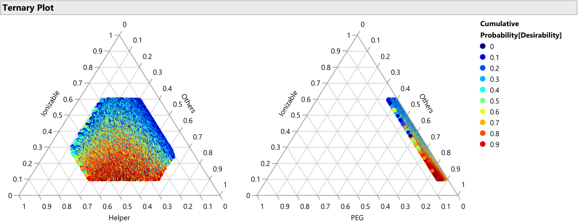
    4. Construct ternary plots for the four lipid factors. In the table, navigate to Graph > Ternary Plot, select the mixture factors for X, Plotting, and click OK. Right-click in one of the resulting graphs, select Row Legend, and then select the predicted response column. Change the Colors dropdown to Jet.
       NOTE: This displays the best and worst performing regions with respect to the lipid factors. Figure 14 shows the percentiles of the joint desirability when considering maximizing Potency (importance=1) and minimizing Size (importance=0.2), while averaging over any factors that are not shown on the ternary plot axes. Figure 15 shows the raw predicted size. It is also reasonable to break down these graphs conditionally on other factors, such as creating a distinct set of ternary plots for each ionizable lipid type with a Local Data Filter (available from the red triangle menu next to Ternary Plot).
    5. Similarly, use Graph > Graph Builder to plot the 50,000 color-coded points (representing unique formulations) against the non-mixture process factors, either individually or jointly, and search for relationships between the response(s) and the factor(s). Look for the factor settings that yield the highest desirability. Explore different combinations of factors in the graphics.
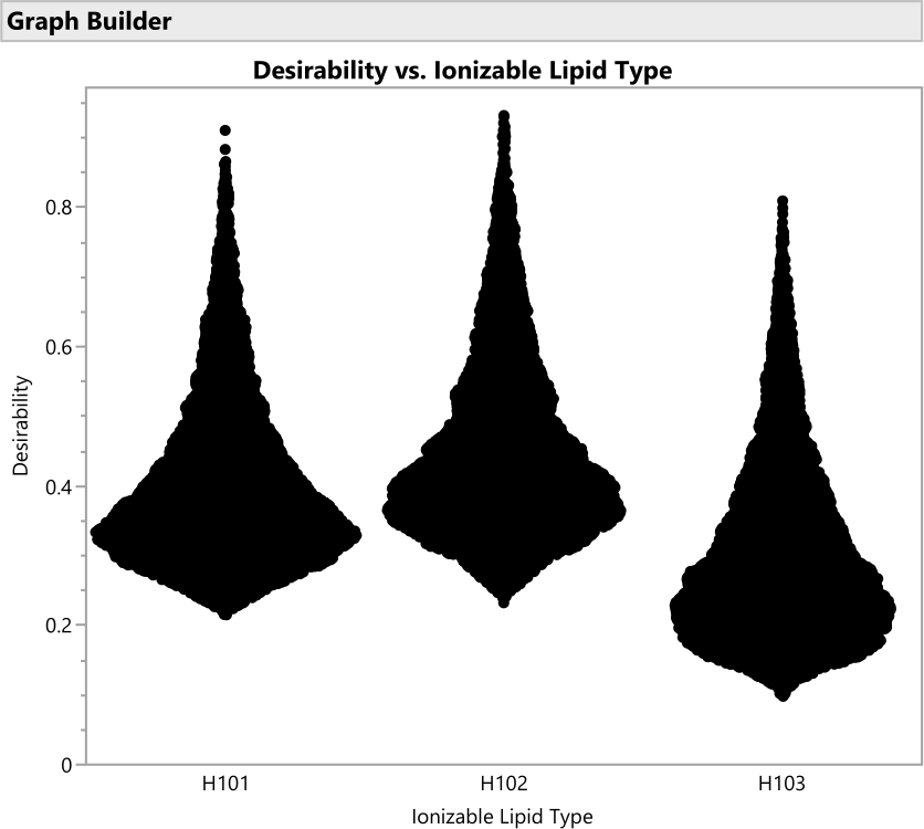
       NOTE: When coloring graphs, use Cumulative Probability[Desirability], but when plotting the desirability on the vertical axis against process factors use the raw Desirability column. The Desirability column can also be placed on an axis of the Graph > Scatterplot 3D visualization along with two other process factors for multivariate exploration. Figure 16 shows the joint desirability of all of the formulations that can be formed with each of the three ionizable lipid types. The most desirable formulations use H102, with H101 providing some potentially competitive alternatives.
    6. Save the Profiler and its remembered settings back to the data table. Click the red triangle next to Profiler and select Save Script > To Data Table….

Figure 8: Observed potency readings from the experiment. The points show the potency values that were observed from the 23 runs; the replicated benchmark runs are shown in green. Please click here to view a larger version of this figure.

Figure 9: Software dialog for initiating the analysis. The candidate effects have been entered along with the target potency response, and the No Intercept option has been unchecked. Please click here to view a larger version of this figure.

Figure 10. Additional dialog for specifying SVEM options. By default, the lipid main effects are forced into the model. Because an intercept is included, we recommend unchecking these boxes in order not to force the effects. Please click here to view a larger version of this figure.

Figure 11: Actual by predicted plot. This figure plots the observed Potency against the value predicted for each formulation by the SVEM model. The correlation need not be as strong as it is in this example, but the expectation is to see at least a moderate correlation and to check for outliers. Please click here to view a larger version of this figure.

Figure 12: Prediction profiler. The top two rows of graphs show the slices of the predicted response function at the optimum formulation (as identified by the SVEM approach). The bottom row of graphs shows the weighted "desirability" of the formulation, which is a function of the last column of graphs which shows that Potency should be maximized, and Size should be minimized. Please click here to view a larger version of this figure.

Figure 13: Three optimal formulation candidates from SVEM-Forward Selection. Changing the relative importance weighting of the responses can lead to different optimal formulations. Please click here to view a larger version of this figure.

Figure 14: Ternary plots for the percentile of desirability. The plot shows the 50,000 formulations color coded by percentile of desirability, where the desirability is set with importance weight of 1.0 for maximizing Potency and 0.2 for minimizing size, these plots show that the optimal region of formulations consists of lower percentages of ionizable lipid and higher percentages of PEG. Please click here to view a larger version of this figure.

Figure 15: Ternary plot for the predicted Size. The plot shows the size predictions from the SVEM model for each of the 50,000 formulations. Size is minimized with higher percentages of helper lipid and maximized with lower percentages of helper. Since the other factors vary freely across the 50,000 plotted formulations, this implies that this relationship holds across the ranges of the other factors (PEG, flow rate, etc.). Please click here to view a larger version of this figure.

Figure 16: Violin plots for the desirability of formulations involving the three different ionizable lipid types. Each of the 50,000 points represents a unique formulation from throughout the allowed factor space. The peaks of these distributions are the maximal values of desirability that are calculated analytically with the prediction profiler. H102 has the largest peak and thus produces the optimal formulation. The SVEM approach to building the model that generates this output automatically filters out statistically insignificant factors: the purpose of this graph is to consider practical significance across the factor levels. Please click here to view a larger version of this figure.

5. Confirmation runs

1. Prepare a table listing the optimal candidates identified previously (Figure 17).
   NOTE: The True Potency and True Size values in Figure 17 are filled in using the simulated generating functions: in practice, these will be obtained by formulating and then measuring the performance of these recipes.
   1. Include the benchmark control with the set of candidate runs that will be formulated and measured.
   2. If any of the formulations from the experiment were found to yield desirable results, perhaps by outperforming the benchmark, select the best to add to the candidate table and retest along with new formulations.
      NOTE: Either manually add desired runs to the candidate table or use the Profiler window's Remembered Settings if these runs are from the previous experiment. Identify the run's row number, navigate to Prediction Profiler > Factor Settings > Set to Data in Row, and input the row number. Then, choose Prediction Profiler > Factor Settings > Remember Settings and label appropriately (e.g., "benchmark" or "best run from the previous experiment").
   3. Right-click on the Remembered Settings table in the Profiler and select Make into Data Table.
      NOTE: Depending on the study's priority and budget, consider running replicates for each confirmation run, especially if replacing the benchmark. Create and analyze each formulation twice, using the average result for ranking. Pay attention to any candidates with a wide response range across the two replicates as this could indicate high process variance.
   4. If necessary due to budget constraints, downselect from the identified candidates to match the experimental budget or to eliminate redundant candidates.
2. Carry out the confirmation runs. Construct the formulations and gather the readouts.
3. Check for consistency between the results from the original experiment and the results for the confirmation batch for benchmarks or other repeated recipes. If there is a large and unexpected shift, then consider what might have contributed to the shift and if it is possible that all runs from the confirmation batch were affected.
4. Compare the performance of the candidate optimal formulations. Explore whether any new candidates outperformed the benchmark.
5. Optional: Add the result of the confirmation runs to the experimental table and rerun the analysis in Section 4.
   NOTE: The next step of the workflow provides instructions for constructing a follow-up study along with these runs if desired.

Figure 17: Table of ten optimal candidates to be run as confirmation runs. The True Potency and True Size have been filled in from the simulation generating functions (without any added process or analytical variation). Please click here to view a larger version of this figure.

6. Optional: Designing a follow-up study to be run concurrently with the confirmation runs

1. Assess the need for a follow-up study considering the following criteria:
   1. Determine if the optimal formulation lies along one of the factor boundaries and if a second experiment is desired to expand at least one of the factor ranges.
   2. Evaluate if the initial experiment used a relatively small run size or relatively large factor ranges and if there is a need to "zoom in" on the identified optimal region with additional runs and updated analysis.
   3. Check if an additional factor is being introduced. This could be a level of a categorical factor such as an additional ionizable lipid or a factor that remained constant in the initial study, for example, buffer concentration.
   4. If none of the above conditions are met, proceed to Step 7.
2. Prepare for additional experimental runs to be carried out concurrently with the confirmation runs.
   1. Define the factor limits ensuring a partial overlap with the region from the initial study. If no overlap exists, a new study must be designed.
   2. Develop the new experimental runs with a space-filling design. Select DOE > Special Purpose > Space Filling Design.
      NOTE: For advanced users, consider a D-optimal design via DOE > Custom Design.
   3. After the space-filling runs are generated, manually incorporate two or three runs from the original experiment that lie within the new factor space. Distribute these runs randomly within the experimental table using the steps described in Section 2 to add rows and then randomize the row order.
      NOTE: These will be used to estimate any shift in the response means between blocks.
   4. Concatenate the confirmation runs and the new space-filling runs into a single table and randomize the run order. Use Tables > Concatenate and then create and sort by a new random column to randomize the run order, as described in Section 2.
3. Formulate the new recipes and collect the results.
4. Concatenate the new experimental runs and results to the original experiment data table, introducing an experiment-ID column to indicate the source of each result. Use Tables > Concatenate and select the option to Create Source Column.
5. Verify that the column properties for each factor display the combined range over both studies: right click on the column header for each factor and examine the Coding and Mixture property ranges, if present.
6. Begin analysis of the new experiment's results.
   1. Include the experiment-ID column as a term in the model to serve as a blocking factor. Ensure this term does not interact with the study factors. Run the Fit Model dialog script saved to the table in Section 4, select the experiment-ID column and click Add to include it in the list of candidate effects.
   2. Run this Fit Model dialog on the concatenated data table to jointly analyze the results from the new experiment and the initial study. Adhere to earlier instructions to generate updated optimal formulation candidates and graphical summaries.
   3. For validation, independently analyze the results from the new experiment, excluding results from the initial experiment. That is, perform the steps described in Section 4 on the new experimental table.
   4. Ensure that optimal formulations identified by these models align closely with those recognized by the joint analysis.
   5. Review graphical summaries to confirm that both the joint and individual analyses of the new experimental results exhibit similar response surface behaviors (meaning that there is a similar relationship between the response(s) and the factors).
   6. Compare the combined and individual analyses of new results with the initial experiment for consistency. Use similar graph structures for comparison and examine the identified optimal recipes for differences.

7. Documenting the study's final scientific conclusions

1. Should the benchmark control change to a newly identified recipe due to the study, log the new setting and specify the design and analysis files that record its origin.
2. Maintain all experimental tables and analysis summaries, preferably with date-stamped file names, for future reference.

Wyniki

This approach has been validated across both broadly classified lipid types: MC3-like classical lipids and lipidoids (e.g., C12-200), generally derived from combinatorial chemistry. Compared to a benchmark LNP formulation developed using a One Factor at a Time (OFAT) method, the candidate formulations generated through our workflow frequently demonstrate potency improvements of 4- to 5-fold on a logarithmic scale, such as shown in the mouse liver luciferase readings in Figure 18. Tab...

Dyskusje

Modern software for the design and analysis of mixture-process experiments makes it possible for scientists to improve their lipid nanoparticle formulations in a structured workflow that avoids inefficient OFAT experimentation. The recently developed SVEM modeling approach eliminates many of the arcane regression modifications and model reduction strategies that may have previously distracted scientists with extraneous statistical considerations. Once the results are collected, the SVEM analysis framework offers an appro...

Materiały

Name	Company	Catalog Number	Comments
JMP Pro 17.1	JMP Statistical Discovery LLC