In Vivo Calcium Imaging of Neuronal Ensembles in Networks of Primary Sensory Neurons in Intact Dorsal Root Ganglia

Summary

This protocol describes the surgical exposure of the dorsal root ganglion (DRG) followed by GCaMP3 (genetically-encoded Ca²⁺ indicator; Green Fluorescent Protein-Calmodulin-M13 Protein 3) Ca²⁺ imaging of the neuronal ensembles using Pirt-GCaMP3 mice while applying a variety of stimuli to the ipsilateral hind paw.

Abstract

Ca²⁺ imaging can be used as a proxy for cellular activity, including action potentials and various signaling mechanisms involving Ca²⁺ entry into the cytoplasm or the release of intracellular Ca²⁺ stores. Pirt-GCaMP3-based Ca²⁺ imaging of primary sensory neurons of the dorsal root ganglion (DRG) in mice offers the advantage of simultaneous measurement of a large number of cells. Up to 1,800 neurons can be monitored, allowing neuronal networks and somatosensory processes to be studied as an ensemble in their normal physiological context at a populational level in vivo. The large number of neurons monitored allows the detection of activity patterns that would be challenging to detect using other methods. Stimuli can be applied to the mouse hindpaw, allowing the direct effects of stimuli on the DRG neuron ensemble to be studied. The number of neurons producing Ca²⁺ transients as well as the amplitude of Ca²⁺ transients indicates sensitivity to specific sensory modalities. The diameter of neurons provides evidence of activated fiber types (non-noxious mechano vs. noxious pain fibers, Aβ, Aδ, and C fibers). Neurons expressing specific receptors can be genetically labeled with td-Tomato and specific Cre recombinases together with Pirt-GCaMP. Therefore, Pirt-GCaMP3 Ca²⁺ imaging of DRG provides a powerful tool and model for the analysis of specific sensory modalities and neuron subtypes acting as an ensemble at the populational level to study pain, itch, touch, and other somatosensory signals.

Introduction

Primary sensory neurons directly innervate the skin and carry somatosensory information back to the central nervous system^1,2. Dorsal root ganglia (DRGs) are cell body clusters of 10,000-15,000 primary sensory neurons^3,4. DRG neurons present diverse size, myelination levels, and gene and receptor expression patterns. Smaller diameter neurons include pain-sensing neurons and larger diameter neurons typically respond to non-painful mechanical stimuli^5,6. Disorders in the primary sensory neurons such as injury, chronic inflammation, and peripheral neuropathies can sensitize these neurons to various stimuli and contribute to chronic pain, allodynia, and pain hypersensitivity^7,8. Therefore, the study of DRG neurons is important in understanding both somatosensation generally and many pain and itch disorders.

Neurons firing in vivo are essential to somatosensation, but until recently, tools to study intact ganglia in vivo have been limited to relatively small numbers of cells⁹. Here, we describe a powerful method for studying the action potentials or activities of neurons on a population level in vivo as an ensemble. The method employs imaging based on cytoplasmic Ca²⁺ dynamics. The Ca²⁺ sensitive fluorescent indicators are good proxies for measuring cellular activity due to the normally low concentration of cytoplasmic Ca²⁺. These indicators have allowed simultaneous monitoring of hundreds to several thousands of primary sensory neurons in mice^{9,10,11,12,13,14,15,16} and rats¹⁷. The method of in vivo Ca²⁺ imaging described in this study can be used to directly observe populational level responses to mechanical, cold, thermal, and chemical stimuli.

The phosphoinositide-binding membrane protein, Pirt is expressed at high levels in almost all (>95%) primary sensory neurons^18,19 and can be used to drive the expression of the Ca²⁺ sensor, GCaMP3, to monitor neuron activity in vivo²⁰. In this protocol, techniques are described for performing in vivo DRG surgery, Ca²⁺ imaging, and analysis in the right side lumbar 5 (L5) DRG of Pirt-GCaMP3 mice¹⁴ using confocal laser scanning microscopy (LSM).

Protocol

All procedures described here were performed in accordance with a protocol approved by the Institutional Animal Care and Use Committee of the University of Texas Health Science Center at San Antonio.

NOTE: Once started, animal surgery (step 1) and imaging (step 2) must be completed in a continuous manner. Data analysis (step 3) may be performed later.

1. Surgery and securing the animal for right side L5 DRG imaging

NOTE: Both male and female Pirt-GCaMP3 C57BL/6J mice 8 weeks of age or older were used in this study. While either sex can be imaged equally well, mice should be at least 8 weeks old due to weak or intermittent Pirt expression in younger mice. The Pirt-GCaMP3 C57BL/6J mice were generated at Johns Hopkins University¹⁴. Either side DRG may be imaged, and other lumbar DRGs (e.g., lumbar 4) may be imaged. The times given are estimates for an experienced surgeon. Occasional technical issues such as increased bleeding may increase the time required.

1. Prepare a sterile saline solution containing 40 mg/mL ketamine and 6 mg/mL xylazine. The total volume should be at least 9 µL/g of body mass for both surgery and euthanasia after imaging.
   CAUTION: Ketamine is harmful if injected, swallowed, or when it comes in contact with the eye. Handle with care.
2. Ensure that all the surgical tools are clean and sterilized by autoclaving or other NIH Guide for the Care and Use of Laboratory Animals-approved method.
3. Between 15 and 25 min before surgery, inject a Pirt-GCaMP3 mouse intraperitoneally (i.p.) with ~2.25 µL of ketamine/xylazine for every gram of body weight (90 mg/kg ketamine, 13.5 mg/kg xylazine). Do not exceed 120 mg/kg ketamine.
4. Within 15 to 25 min after injection of anesthesia (step 1.3), check whether the mouse has reached the surgical plane of anesthesia by pinching the contralateral hind paw (not the ipsilateral/right hind paw). The absence of hindlimb withdrawal reflex ensures that a surgical plane of anesthesia is achieved.
   NOTE: Hindlimb withdrawal reflex is used throughout the experiment to monitor anesthesia. Always use the contralateral hind paw.
5. Place the mouse on a heated pad to maintain the body temperature at 37 °C.
   NOTE: It may be helpful to hold the mouse's head in place with a stereotaxic frame (see Table of Materials), or another frame based on the researcher's preference.
6. Locate the lumbar enlargement by feeling for the mouse's pelvic bone. Shave the back of the mouse above the lumbar enlargement area. This step should take ~90 s.
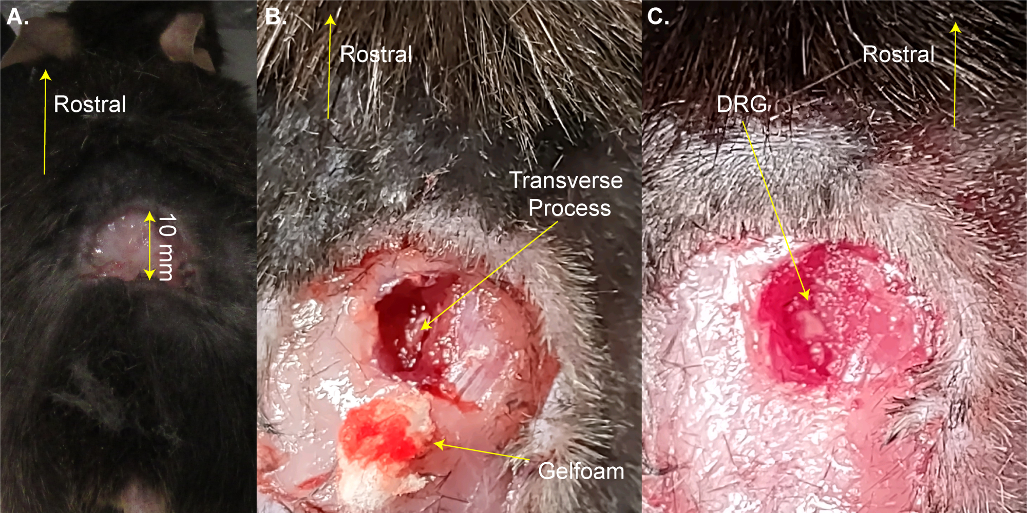
   NOTE: The mouse can be briefly removed from the heated pad for shaving.
7. Make a three-sided rectangular incision (8 mm x 20 mm) above the lumbar enlargement using scissors and fold the skin away with forceps (Figure 1A). This step takes ~2 min.
   NOTE: Researchers may also use hemostat forceps or a retractor to hold the incision open. This is not a survival surgery, so additional cleaning of the surgical area is not necessary; however, it may be done using povidone-iodine. The largest acceptable incision size is given here. A smaller incision is preferable to a larger incision.
8. Use the 13 mm spring dissection scissors to make 3-4 mm incisions on the right side of the spine. Use scissors to cut back the skin and muscles to the sides in order to expose the spine (Figure 1B). This step takes ~3 min.
9. Use 8 mm scissors to clean the transverse process of the right-side L5 DRG by cutting away the muscle and connective tissue while trying to minimize bleeding. Use cotton and/or gelfoam to absorb the blood. The L5 vertebra is the first vertebra rostral to the pelvice bone.
   NOTE: This step takes ~3 min and may take extra time if the animal bleeds more than normal.
10. Cut open the right-side L5 transverse process using Friedman-Pearson rongeurs or strong fine forceps. Be careful to not touch the DRG (Figure 1C).
    NOTE: This step takes ~2 min but may take extra time if the animal bleeds more than normal.
11. Do not proceed until bleeding stops completely. Prevent bleeding onto the DRG surface using gel foam or cotton. This step step takes 1-4 min.
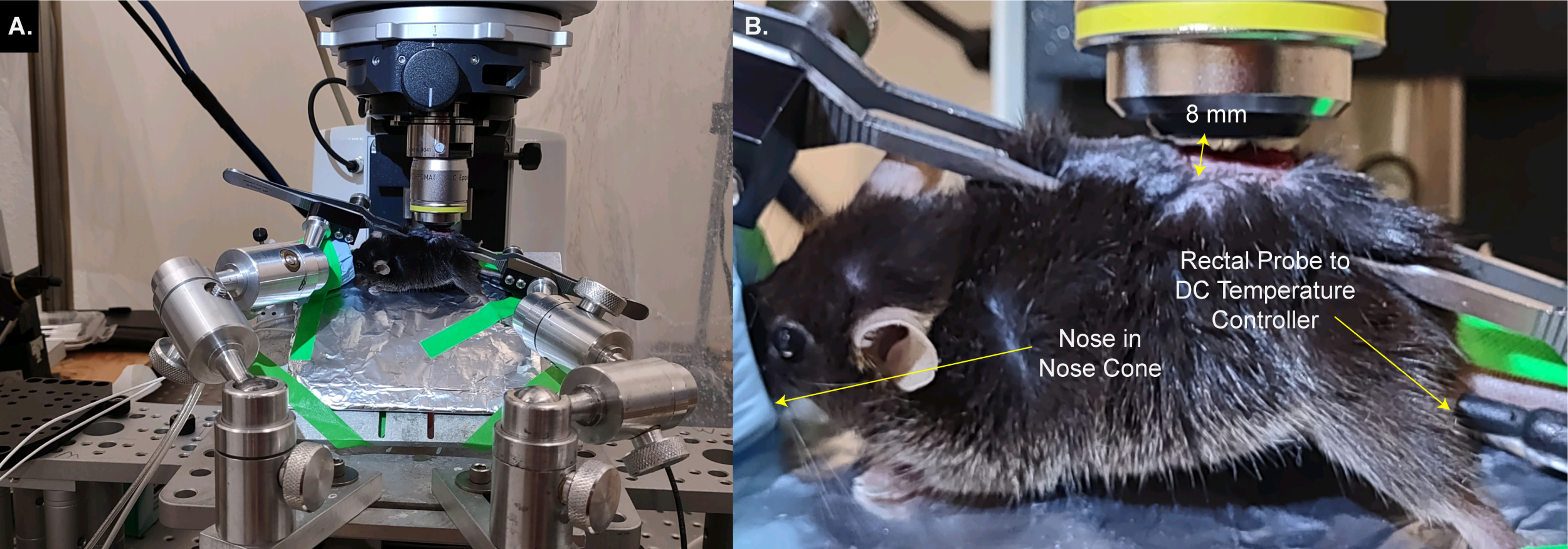
12. Move the mouse and heating pad onto the custom stage (Figure 2A,B). Use stage tape to secure the animal and heating pad in place. Place the animal's nose in the nose cone so that the animal can receive continuous isoflurane anesthesia. Secure the right hindpaw sticking out off the stage so that the stimuli can be easily applied to the paw. This step takes 3 min.
13. Secure the spine in place with the stage clamps over the skin on the vertebrae and/or the pelvic bone just rostral and caudal to the L5 DRG. Adjust the clamps and the stage to make the surface of the DRG as level as possible (Figure 2B,C).
    NOTE: It may be necessary to trim the tissue lying between the DRG and the objective.
14. Place the stage below the microscope so that the objective is 8 mm directly above the DRG when lowered (Figure 3A,B). Insert the rectal thermometer.
    NOTE: The distance from the DRG to the objective may vary based on the objective, the microscope, and the animal.
15. Connect the power lines to the heating pad and the rectal thermometer. Connect the nose cone to the isoflurane gas lines.

Figure 1: Example of DRG exposure surgery. (A) A small area was shaved and the skin was cut and folded back. The incision is ~10 mm on the rostral-caudal axis. (B) An incision was made on the right side of the spinal column and muscle and connective tissue were cut away, exposing the L5 right side transverse process. Blood was absorbed with gelfoam. (C) The transverse process was cleaned and the bone over the DRG was removed. Please click here to view a larger version of this figure.

Figure 2: Mounting the mouse on a custom stage for DRG imaging. (A) The custom stage is shown. It consists of a base plate and a plate for the animal. The animal mounting plate is on a locking ball and socket swivel joint. A nose cone with lines for delivering oxygen / isoflurane mixture and a waste gas line along with an aluminum foil wrapped heating pad are taped to the animal mounting plate. Two arms, each made from three locking ball and socket swivel joints, are bolted to the base plate. Each arm has a clamp made from forceps with a screw for tightening and loosening. (B) The animal is mounted on the animal mounting plate. Its nose is placed in the nose cone. Clamps are placed over the skin holding the spinal column and pelvic bone. The right (ipsilateral) hindpaw is taped to stick out for easy access for applying stimuli. (C) A closeup image of the clamped spinal column and pelvic bone. Please click here to view a larger version of this figure.

Figure 3: Animal on custom stage is placed below the microscope objective. (A) A wide angle view of the stage, animal, and microscope. Wires to the DC temperature controller and lines to oxygen / isoflurane intake and waste gas line are visible on the left. (B) A closeup view of the animal below the microscope objective. The DRG is ~8 mm below the objective. The rectal thermometer is inserted and the nose is inside the nose cone. Please click here to view a larger version of this figure.

2. DRG imaging

1. Use an upright confocal microscope 10x/0.4 DIC objective and the associated software (see Table of Materials) for imaging. Use the green filter (FITC) settings: excitation 495 nm, emission 519 nm, detection wavelength 500-580 nm, GaAsP-Pmt1 imaging device, GaAsP-PMT detector.
   NOTE: For other microscopes use the manufacturer's recommended settings.
2. Find the surface of the DRG with the microscope. Adjust the clamps on the stage such that the DRG surface is as level as possible and that the maximum surface area is visualized in the focal plane.
   NOTE: The choice of objective may vary depending on the microscope used and the user preference. The choice of software depends on the microscope. A level DRG results in clearer images, allows the software to construct clearer movies, allows imaging of more neurons, and makes analysis easier and more accurate.
3. Supply 1%-1.5% isoflurane in oxygen flow to the nose cone to ensure the mouse remains anesthetized. Monitor the animal carefully throughout the procedure to maintain isoflurane anesthesia without overdosing.
   NOTE: The amount of isoflurane necessary to maintain anesthesia may vary by individual animal and stimulus. Usually, 1.5% is sufficient. If the animal moves during stimulus, isoflurane should be increased. If breathing becomes shallow, isoflurane should be decreased. Before each stimulus, test the hindlimb withdraw reflex on the contralateral hind paw.
   CAUTION: Isoflurane can be harmful or cause dizziness or drowsiness if inhaled. Avoid inhalation and use only in a well-ventilated area.
4. Load the microscope rapid scanning protocol.
   1. Use the typical settings for rapid scanning: voxel size 2.496 µm x 2.496 µm x 16 µm, 512 x 512 pixels, 10 optical slice Z-stack, 1 airy unit (AU)/32 µm, 1% 488 nm laser power 5 mW, pixel time 1.52 µs, line time 0.91 ms, frame time 465 ms, LSM scan speed 8, bidirectional scanning, GaAsP-PMT detector gain 650 V, digital gain 1. Optimal settings may vary by microscope and animal.
   2. To set up a rapid scanning protocol, click on the Acquisition tab. Under Acquisition Parameters, click on the Frames tab. Click on Presets > 512 x 512 to set the microscope to record a 512 pixel x 512 pixel image. This will in turn set the X and Y values of the voxel size based on the image size, which is determined by the microscope software.
   3. Under Acquisition Parameters, click on the Channels tab. Click on the Track2 box. Use the drop-down menu beside the Track2 box to select Green (FITC). A new tab will open below Track2.
   4. Beside Lasers, click on the 488 box. This will set the excitation and emission wavelengths.
   5. Beside the 488 nm slider, set Laser Power to 1%. Click on the 1 AU button to set the aperature for 1 Airy unit. Under FITC, set Master Gain to 650 V, Digital Offset to 0, and Digital Gain to 1.
   6. Under the Acquisition tab, check the Z-Stack box. Click on the Live button to view a live image of the ganglion. Turn the focal plane knob up until only a small arc of neurons are visible.
   7. Under Acquisition Parameters, click on the Z-Stack tab > Set Last button. Turn the focal plane knob down until only a small arc of neurons are visible. Under Acquisition Parameters, click on the Z-Stack tab > Set First button. Click on the Live button to turn off the live image.
   8. Under Acquisition Parameters, click on the Z-Stack tab. Fill in the Slices field with 10. This will set 10 optical slices and automatically determine the voxel depth.
   9. Under the Acquisition tab, click on the Time Series box. A new Time Series tab will appear under Acquisition Parameters. Click on the Time Series tab > Cycles field with the number of cycles you wish to take next. In this case, it is 8.
   10. Set the scan speed and direction. Under Acquisition Parameters, Acquisition Mode tab > > Direction > Double Headed Arrow for birdirectional scanning. Select Acquisition Mode tab > Frame > Scan Speed Slider > 8.
       NOTE: Normally one can load settings of a prior experiment and only have to adjust the laser power if the image is too bright or dim and adjust the Z-Stack Set Last and Set First.
5. Take a short 8 cycle scan of the DRG by clicking on Start Experiment under the Acquisition tab. Create a movie by making an orthogonal projection of scans (one scan per frame) over time and manually check for image clarity and imaging artifacts such as "waves" of brightness crossing the DRG. Adjust clamp position and optical section thickness and repeat this step until a clear, high quality movie is achieved.
   NOTE: This step should be repeated if the animal moves or is moved by the investigator. Problems to look for include areas of the ganglion (not just single neurons) appearing to become lighter and darker over the course of the experiment creating a wavy appearance or causing areas to disappear or become brighter. Movement greater than about half of a small neuron’s diameter (<20 µm) is another major problem. Wavyness can often be fixed by bringing the first and last position of the Z-Stack closer together (see step 2.4.4 above) and narrowing the optical slice thickness. Movie 1 provides an example of a wavy ganglia prior to leveling and setting the correct optical slice thickness. Movie 2 is after correcting leveling and optical slice thickness. The difference is subtle, but it has a tremendous effect on analysis.
6. Load the microscope high resolution scanning protocol.
   1. Use the typical settings for high resolution scanning: voxel size 1.248 µm x 1.248 µm x 14 µm, 1024 x 1024 pixels, 6 optical slice Z-stack, 1.2 airy unit (AU)/39 µm, 5% 488 nm laser power/25 mW, pixel time 2.06 µs, line time 4.95 ms, frame time 5.06 s, LSM scan speed 6, bidirectional scanning, GaAsP-PMT detector gain 650 V, digital gain 1. Optimal settings may vary by microscope and animal.
   2. To set up a high resolution scanning protocol, click on the Acquisition tab. Under Acquisition Parameters, click on the Frames tab. Click on Presets > 1024 x 1024 to set the microscope to record a 1024 pixel x 1024 pixel image. This will in turn set the X and Y values of the voxel size based on the image size, which is determined by the microscope software.
   3. Under Acquisition Parameters, click on the Channels tab. Click on the Track2 box. Use the drop-down menu beside the Track2 box to select Green (FITC). A new tab will open below Track2.
   4. Beside Lasers, click on the 488 box. This will set the excitation and emission wavelengths. Click on the High Intensity Laser Range box.
   5. Beside the 488 nm slider, set Laser Power to 5%. Click on the 1 AU button to set the aperature for 1 Airy unit. Under FITC set Master Gain to 650 V, Digital Offset to 0, and Digital Gain to 1.
   6. Under the Acquisition tab, check the Z-Stack box. Click on the Live button to view a live image of the ganglion. Turn the focal plane knob up until only a small arc of neurons are visible.
   7. Under Acquisition Parameters, click on the Z-Stack tab > Set Last button. Turn the focal plane knob down until only a small arc of neurons are visible. Under Acquisition Parameters, click on the Z-Stack tab > Set First button. Click on the Live button to turn off the live image.
   8. Under Acquisition Parameters, click on the Z-Stack tab. Fill in the Slices field with 6. This will set 6 optical slices and automatically determine voxel depth.
   9. Under the Acquisition tab, make sure the Time Series box is unchecked (no time series).
   10. Set the scan speed and direction. Under Acquisition Parameters, click on the Acquisition Mode tab > Frame > Presets > 1024 x 1024. Select the Acquisition Mode tab > Frame > Direction > Double Headed Arrow for bidirectional scanning. Select the Acquisition Mode tab > Frame > Scan Speed Slider > 6.
   11. If cells are labeled with td-Tomato, set the microscope to scan the red channel 592 nm excitation/614 nm emission, detection wavelength 600-700 nm in addition to the green channel. Set this by going to Acquisition Parameters and click on the Channels tab > Track1 box. Use the drop down menu beside the Track1 box to select Red (Texas Red). Follow the same process as in step 2.6.3, except click on the 561 box instead of the 488 box. Set Laser Power to 1%. Td-Tomato is much brighter than GCaMP3 and requires lower laser power.
7. Make a high-resolution image of the DRG by clicking on the Start Experiment button under the Acquisition tab.
8. Load the microscope rapid scanning protocol (see step 2.4). Record spontaneous activity in the DRG for 80 cycles (approximately 10 min). Generate an orthogonal projection movie and verify that the image is of sufficient quality for analysis.
   NOTE: Quality considerations are the same as in step 2.5.
9. For applying stimuli, set the microscope to perform 15-20 scans. Wait for scans 1-5 to complete to produce the baseline. Apply the stimulus during scans 6-10. Wait at least 5 min following each stimulus before applying the next stimulus to prevent desensitization.
   NOTE: Mechanical stimuli should be applied first, and then cold, thermal, and chemical stimuli. Weaker stimuli (e.g., low mechanical force, temperatures closer to room temperature) should be applied before stronger stimuli (e.g., higher mechanical force, temperatures farther from room temperature). When applying stimuli, be sure not to cause any movement of the DRG. For strong thermal stimuli in particular, it is often necessary to apply 2% isoflurane for 1-2 min before starting the stimulus. On the microscope used in this study, each scan can be heard clearly, such that the researcher can easily identify the end of the scan, allowing stimulus application immediately after scan 5. However, any method that facilitates application of stimuli at a consistent time point will work.
10. For a mechanical press, hold the algometer's pincher with the paw between the paddles without touching the paw, and pinch starting immediately after the end of scan 5 and stopping immediately after scan 10. Monitor the press force with an algometer (see Table of Materials). Keep the press force as close to the desired force (here we use a 100 g press stimulus) as possible and make sure it does not exceed 10 g over the desired force.
    NOTE: One can detect stimuli with as little as 0.07 g von Frey filaments and as much as 600 g press force.
11. For cold and thermal stimuli, cool or heat a beaker of water to just below (for cold) or above (for thermal) the desired temperature and start scanning. Here, use a 45 °C stimulus. When the water is the correct temperature, apply the stimulus immediately after scan 5 by immersing the paw in the water. Pull the beaker away immediately after scan 10.
    NOTE: The temperature should be within 1 °C of the desired temperature on scan 5. If the beaker temperature is incorrect, do not apply the stimulus because this could desensitize the neurons. Instead recool or reheat the water and try again. We have measured temperatures as low as 0 °C (ice water) and as high as 95 °C. However, remember that temperatures above 50 °C may damage tissues and confound later experiments. Similarly, some chemicals (e.g. tetrodotoxin, capsaicin) are irreversible or cannot be washed out and can prevent further experiments on the animal.
12. After all stimuli have been applied and recorded, euthanize the animal by overdosing with ketamine/xylazine (200 mg/kg ketamine, 30 mg/kg xylazine, or 5 µL per gram body mass of solution prepared in step 1.1) followed by decapitation.

3. Data analysis

1. Open the image files by dragging and dropping into ImageJ. After opening the file, select the image type under Image > Type > RGB color.
   NOTE: The StackReg²¹ plugin under Plugins > StackReg is useful for correcting and aligning movement artifacts. ImageJ can read most microscope software file formats. The choice of image type depends on user preference. RGB simplifies producing color images for publication. Software packages from the microscope manufacturer or cytoNet²² may aid in analysis, as well. It is not necessary to download, install, and use StackReg, but it is recommended.
2. Use the region of interest (ROI) tool to select active neurons under Analyze > Tool > ROI Manager. Draw ROIs using the ellipse or rectangle tools on the toolbar and place them in the ROI file by pressing the Add button under Add on the ROI manager window, or by pressing the "t" key.
   NOTE: Be sure to frequently save the ROI file. Users can always restore ROIs by dragging and dropping an ROI file into ImageJ and clicking on the Show All box at the bottom of the ROI Manager window. Saving as an overlay is not recommended. From experience, saving as an ROI.zip file simplifies analysis.
3. Under Analyze > Set Measurements, make sure the mean gray value option is checked; uncheck all other boxes under Set Measurements. Use the multi-measure tool on the ROI manager menu to calculate intensity within the ROIs. Measure intensity using the ROI window under More > Multimeasure.
   NOTE: Sometimes adjacent neurons will be too close together to draw separate ROIs. These neurons cannot be used to measure transient intensity, but may be included in counts of activating neurons.
4. Save the CSV file generated by Multimeasure and open the CSV file with any spreadsheet software.
   NOTE: See Supplementary File 1 for an example spreadsheet template to aid analysis.
5. Calculate Ca²⁺ transient intensity as ΔF / F₀ = (F_t- F₀) / F₀, where F_t is the pixel intensity in an ROI at the time point of interest, and F₀ is the baseline intensity determined by averaging the intensities of either the 2-4 frames before the Ca²⁺ transient for spontaneous activity or the first 1-5 frames of the ROI for Ca²⁺ transients occurring during stimulation. Exclude any neurons producing Ca²⁺ peaks before the stimulus and do not analyze activity after the stimulus ends.
6. For Ca²⁺ transient intensity analysis, randomly sample approximately equal numbers of neurons from each ganglion to avoid skewing the data toward ganglia that produced the largest number of responding neurons. Exclude peaks where ΔF / F₀ < 0.15.
   NOTE: There are alternative published methods of analysis and inclusion/exclusion of neurons^{11,12,23,24,25,26,27,28}.
7. Measure neuron diameters using the line tool on the toolbar in ImageJ. Calculate the average diameter from the lines drawn along the longest and shortest diameters.

Results

Figure 4: Representative images of L5 dorsal root ganglia of Pirt-GCaMP3 mice. (A,D) Single frame high resolution scans of L5 dorsal root ganglia of Pirt-GCaMP3 mice are shown. (B,E). Average intensity projections of 15 frames of Pirt-GCaMP3 L5 DRG ganglia from panel A and panel D, respectively...

Discussion

Persistent pain is present in a wide range of disorders, debilitating and/or reducing the quality of life for about 8% of people²⁹. Primary sensory neurons detect noxious stimuli on the skin, and their plasticity contributes to persistent pain⁸. While neurons can be studied in cell culture and explants, doing so removes them from their normal physiological context. Surgical exposure of the DRG, followed by Pirt-GCaMP3 Ca²⁺ imaging, permits the study of primary se...

Materials

Name	Company	Catalog Number	Comments
Anased Injection (Xylazine)	Covetrus, Akorn	33197
C Epiplan-Apochromat 10x/0.4 DIC	Cal Zeiss	422642-9900-000
Cotton Tipped Applicators	McKesson	24-106-1S
Curved Hemostat	Fine Science Tools	13007-12
DC Temperature Controller	FHC	40-90-8D
DC Temperature Controller Heating Pad	FHC	40-90-2-05
Dumont Ceramic Coated Forceps	Fine Science Tools	11252-50
FHC DC Temperature Controller	FHC	40-90-8D
Fluriso (Isoflurane)	MWI Animal Health, Piramal Group	501017
Friedman-Pearson Rongeurs	Fine Science Tools	16221-14
GelFoam	Pfizer	09-0353-01
Ketaset (Ketamine)	Zoetis	KET-00002R2
Luminescent Green Stage Tape	JSITON/ Amazon	B803YW8ZWL
Matrx VIP 3000 Isoflurane Vaporizer	Midmark	91305430
Micro dissecting scissors	Roboz	RS-5882
Micro dissecting spring scissors	Fine Science Tools	15023-10
Micro dissecting spring scissors	Roboz	RS-5677
Mini Rectal Thermistor Probe	FHC	40-90-5D-02
Operating scissors	Roboz	RS-6812
Pirt-GCaMP3 C57BL/6J mice	Johns Hopkins University	N/A	Either sex can be imaged equally well. Mice should be at least 8 weeks old due to weak or intermittent Pirt promoter expression in younger mice.
SMALGO small animal algometer	Bioseb In vivo Research Instruments	BIO-SMALGO
Stereotaxic frame	Kopf Model 923-B	923-B
td-Tomato C57BL/6J mice	Jackson Laboratory	7909
Top Plate, 6 in x 10 in	Newport	290-TP
TrpV1-Cre C57BL/6J mice	Jackson Laboratory	17769
Zeiss LSM 800 confocal microscope	Cal Zeiss	LSM800
Zeiss Zen 2.6 Blue Edition Software	Cal Zeiss	Zen (Blue Edition) 2.6

References

- Rivero-Melián, C., Grant, G. Distribution of lumbar dorsal root fibers in the lower thoracic and lumbosacral spinal cord of the rat studied with choleragenoid horseradish peroxidase conjugate. The Journal of Comparative Neurology. 299 (4), 470-481 (1990).
- Wessels, W. J., Marani, E. A rostrocaudal somatotopic organization in the brachial dorsal root ganglia of neonatal rats. Clinical Neurology and Neurosurgery. 95, 3-11 (1993).
- Schmalbruch, H. The number of neurons in dorsal root ganglia L4-L6 of the rat. The Anatomical Record. 219 (3), 315-322 (1987).
- Sørensen, B., Tandrup, T., Koltzenburg, M., Jakobsen, J. No further loss of dorsal root ganglion cells after axotomy in p75 neurotrophin receptor knockout mice. The Journal of Comparative Neurology. 459 (3), 242-250 (2003).
- Basbaum, A. I., Woolf, C. J. Pain. Current Biology. 9 (12), 429-431 (1999).
- Liu, Y., Ma, Q. Generation of somatic sensory neuron diversity and implications on sensory coding. Current Opinion in Neurobiology. 21 (1), 52-60 (2011).
- Basbaum, A. I., Bautista, D. M., Scherrer, G., Julius, D. Cellular and molecular mechanisms of pain. Cell. 139 (2), 267-284 (2009).
- Stucky, C. L., Mikesell, A. R. Cutaneous pain in disorders affecting peripheral nerves. Neuroscience Letters. 765, 136233 (2021).
- Iseppon, F., Linley, J. E., Wood, J. N. Calcium imaging for analgesic drug discovery. Neurobiology of Pain. 11, 100083 (2022).
- Chen, Z., et al. Adjacent intact nociceptive neurons drive the acute outburst of pain following peripheral axotomy. Scientific Reports. 9 (1), 7651 (2019).
- Chisholm, K. I., Khovanov, N., Lopes, D. M., La Russa, F., McMahon, S. B. Large scale in vivo recording of sensory neuron activity with GCaMP6. eNeuro. 5 (1), (2018).
- Emery, E. C., et al. In vivo characterization of distinct modality-specific subsets of somatosensory neurons using GCaMP. Science Advances. 2 (11), 1600990 (2016).
- Ishida, H., et al. In vivo calcium imaging visualizes incision-induced primary afferent sensitization and its amelioration by capsaicin pretreatment. The Journal of Neuroscience. 41 (41), 8494-8507 (2021).
- Kim, Y. S., et al. Coupled activation of primary sensory neurons contributes to chronic pain. Neuron. 91 (5), 1085-1096 (2016).
- MacDonald, D. I., et al. Silent cold-sensing neurons contribute to cold allodynia in neuropathic pain. Brain. 144 (6), 1711-1726 (2021).
- Wang, F., et al. Sensory afferents use different coding strategies for heat and cold. Cell Reports. 23 (7), 2001-2013 (2018).
- Kucharczyk, M. W., et al. The impact of bone cancer on the peripheral encoding of mechanical pressure stimuli. Pain. 161 (8), 1894-1905 (2020).
- Kim, A. Y., et al. a phosphoinositide-binding protein, functions as a regulatory subunit of TRPV1. Cell. 133 (3), 475-485 (2008).
- Kim, Y. S., et al. Central terminal sensitization of TRPV1 by descending serotonergic facilitation modulates chronic pain. Neuron. 81 (4), 873-887 (2014).
- Tian, L., et al. Imaging neural activity in worms, flies and mice with improved GCaMP calcium indicators. Nature Methods. 6 (12), 875-881 (2009).
- Thévenaz, P., Ruttimann, U. E., Unser, M. A pyramid approach to subpixel registration based on intensity. IEEE Transactions on Image Processing. 7 (1), 27-41 (1998).
- Mahadevan, A. S., et al. cytoNet: Spatiotemporal network analysis of cell communities. PLoS Computational Biology. 18 (6), 1009846 (2022).
- Barretto, R. P., et al. The neural representation of taste quality at the periphery. Nature. 517 (7534), 373-376 (2015).
- Leijon, S. C. M., et al. Oral thermosensing by murine trigeminal neurons: modulation by capsaicin, menthol and mustard oil. The Journal of Physiology. 597 (7), 2045-2061 (2019).
- Sekiguchi, K. J., et al. Imaging large-scale cellular activity in spinal cord of freely behaving mice. Nature Communications. 7, 11450 (2016).
- Wu, A., Dvoryanchikov, G., Pereira, E., Chaudhari, N., Roper, S. D. Breadth of tuning in taste afferent neurons varies with stimulus strength. Nature Communications. 6, 8171 (2015).
- Ran, C., Hoon, M. A., Chen, X. The coding of cutaneous temperature in the spinal cord. Nature Neuroscience. 19 (9), 1201-1209 (2016).
- Yarmolinsky, D. A., et al. Coding and plasticity in the mammalian thermosensory system. Neuron. 92 (5), 1079-1092 (2016).
- Torrance, N., Smith, B. H., Bennett, M. I., Lee, A. J. The epidemiology of chronic pain of predominantly neuropathic origin. Results from a general population survey. The Journal of Pain. 7 (4), 281-289 (2006).
- Shannonhouse, J., et al. Meclizine and metabotropic glutamate receptor agonists attenuate severe pain and Ca(2+) activity of primary sensory neurons in chemotherapy-induced peripheral neuropathy. The Journal of Neuroscience. 42 (31), 6020-6037 (2022).
- Luiz, A. P., et al. Cold sensing by Na(V)1.8-positive and Na(V)1.8-negative sensory neurons. Proceedings of the National Academy of Sciences of the United States of America. 116 (9), 3811-3816 (2019).
- Hartung, J. E., Gold, M. S. GCaMP as an indirect measure of electrical activity in rat trigeminal ganglion neurons. Cell Calcium. 89, 102225 (2020).
- Chung, M. K., Wang, S., Oh, S. L., Kim, Y. S. Acute and chronic pain from facial skin and oral mucosa: Unique neurobiology and challenging treatment. International Journal of Molecular Sciences. 22 (11), 5810 (2021).
- Chan, S. L., Mayne, M., Holden, C. P., Geiger, J. D., Mattson, M. P. Presenilin-1 mutations increase levels of ryanodine receptors and calcium release in PC12 cells and cortical neurons. The Journal of Biological Chemistry. 275 (24), 18195-18200 (2000).
- Sierra, D. A., Popov, S., Wilkie, T. M. Regulators of G-protein signaling in receptor complexes. Trends in Cardiovascular Medicine. 10 (6), 263-268 (2000).
- Yoshihara, K., et al. Astrocytic Ca(2+) responses in the spinal dorsal horn by noxious stimuli to the skin. Journal of Pharmacological Sciences. 137 (1), 101-104 (2018).
- Tan, C. H., McNaughton, P. A. The TRPM2 ion channel is required for sensitivity to warmth. Nature. 536 (7617), 460-463 (2016).
- Akemann, W., Mutoh, H., Perron, A., Rossier, J., Knöpfel, T. Imaging brain electric signals with genetically targeted voltage-sensitive fluorescent proteins. Nature Methods. 7 (8), 643-649 (2010).
- Gong, Y., et al. High-speed recording of neural spikes in awake mice and flies with a fluorescent voltage sensor. Science. 350 (6266), 1361-1366 (2015).
- Grewe, B. F., Langer, D., Kasper, H., Kampa, B. M., Helmchen, F. High-speed in vivo calcium imaging reveals neuronal network activity with near-millisecond precision. Nature Methods. 7 (5), 399-405 (2010).
- Harada, K., et al. Red fluorescent protein-based cAMP indicator applicable to optogenetics and in vivo imaging. Scientific Reports. 7 (1), 7351 (2017).
Reprints and Permissions
Request permission to reuse the text or figures of this JoVE article
Request PermissionThis article has been published
Video Coming Soon
Copyright © 2025 MyJoVE Corporation. All rights reserved