Microsatellite DNA Genotyping and Flow Cytometry Ploidy Analyses of Formalin-fixed Paraffin-embedded Hydatidiform Molar Tissues

Summary

Hydatidiform moles are abnormal human pregnancies with heterogeneous aetiologies that can be classified according to their morphological features and parental contribution to the molar genomes. Here, protocols of multiplex microsatellite DNA genotyping and flow cytometry of formalin-fixed paraffin-embedded molar tissues are described in detail, together with results’ interpretation and integration.

Abstract

Hydatidiform mole (HM) is an abnormal human pregnancy characterized by excessive trophoblastic proliferation and abnormal embryonic development. There are two types of HM based on microscopic morphological evaluation, complete HM (CHM) and partial HM (PHM). These can be further subdivided based on the parental contribution to the molar genomes. Such characterization of HM, by morphology and genotype analyses, is crucial for patient management and for the fundamental understanding of this intriguing pathology. It is well documented that morphological analysis of HM is subject to wide interobserver variability and is not sufficient on its own to accurately classify HM into CHM and PHM and distinguish them from hydropic non-molar abortions. Genotyping analysis is mostly performed on DNA and tissues from formalin-fixed paraffin-embedded (FFPE) products of conception, which have less than optimal quality and may consequently lead to wrong conclusions. In this article, detailed protocols for multiplex genotyping and flow cytometry analyses of FFPE molar tissues are provided, along with the interpretation of the results of these methods, their troubleshooting, and integration with the morphological evaluation, p57^KIP2 immunohistochemistry, and fluorescence in situ hybridization (FISH) to reach a correct and robust diagnosis. Here, the authors share the methods and lessons learned in the past 10 years from the analysis of approximately 400 products of conception.

Introduction

A hydatidiform mole (HM) is an abnormal human pregnancy characterized by abnormal embryonic development, hyperproliferation of the trophoblast, and hydropic degeneration of chorionic villi (CV). Historically, HM used to be divided into two types, complete HM (CHM) and partial HM (PHM) based only on morphological evaluation¹. However, it has been shown that morphological evaluation alone is not sufficient to classify HM into the two subtypes (CHM and PHM) and distinguish them from non-molar miscarriages^2,3,4.

Because CHM and PHM have different propensities to malignancies, it is therefore important to accurately determine the genotypic type of HM to provide appropriate follow-up and management to the patients. Consequently, in the past decades, several methodologies have been developed and evolved for the purpose of identifying the parental contribution to the molar tissues and reaching a correct classification of HM. These include karyotype analysis, chromosomal banding polymorphism, human leukocyte antigen (HLA) serological typing, restriction fragment length polymorphism, variable number of tandem repeats, microsatellite genotyping, flow cytometry, and p57^KIP2 immunohistochemistry. This has allowed accurate subdivision of HM conceptions based on the parental contribution to their genomes, as follows: CHM, which are diploid androgenetic monospermic or diploid androgenetic dispermic, and PHM, which are triploid, dispermic in 99% and monospermic in 1% of the cases^5,6,7,8. Furthermore, there is another genotypic type of HM that emerged in the past two decades, which is diploid biparental. The latter is mostly recurrent and may affect a single family member (simplex cases) or at least two family members (familial cases). These diploid biparental moles are mostly caused by recessive mutations in NLRP7 or KHDC3L in the patients^9,10,11,12. Diploid biparental HM in patients with recessive mutations in NLRP7 may be diagnosed as CHM or PHM by morphological analysis and this appears to be associated with the severity of the mutations in the patients^13,14. In addition to the classification of HM according to their genotypes, the introduction and use of several genotyping methods allowed the distinction of the various molar entities from non-molar miscarriages, such as aneuploid diploid biparental conceptions and other types of conceptions^5,15. Such conceptions may have some trophoblast proliferation and abnormal villous morphology that mimic, to some extent, some morphological features of HM.

The purpose of this article is to provide detailed protocols for multiplex genotyping and flow cytometry of formalin-fixed paraffin-embedded (FFPE) tissues, and comprehensive analyses of the results of these methods and their integration with other methods for correct and conclusive diagnosis of molar tissues.

Protocol

This research study was approved by the McGill Institutional Review Board. All patients provided written consent to participate in the study and to have their FFPE products of conception (POCs) retrieved from various pathology departments.

NOTE: While there are several methods for genotyping and ploidy determination by flow cytometry, the protocols provided here describe one method of analysis using one platform for each.

1. Genotyping

1. Selection of the best FFPE block
   1. For each FFPE product of conception (POC), prepare 4 µm-thick hematoxylin and eosin (H&E) stained sections as described in sections 1.2 and 1.3, one for each available block, for morphological evaluation by microscopy.
   2. Using the H&E slides and a light microscope, select the FFPE block that has the largest amount of chorionic villi (CV), and if possible, the block that has CV separate from, and not intermingled with, maternal tissues.
2. Sectioning
   1. Place the chosen block on ice for 15 min to facilitate the sectioning.
   2. Adjust the microtome to cut sections that are 4 µm thick for microscopic morphological evaluation and 10 µm thick for DNA extraction.
   3. Place the cold block in the microtome and cut one section from each block for H&E staining and 10−30 sections from the chosen block, depending on the amount of CV in the block, for DNA extraction.
      NOTE: For blocks that are full of CV, 10 sections are sufficient for DNA extraction. If only about 10% of the block contains CV while the rest are maternal tissues, then 20−30 sections are needed to ensure sufficient amounts of DNA.
   4. Using forceps, transfer each section to a 45 °C water bath. Pick up the section from the water bath with a positively charged slide (Table of Materials) that is previously labelled with the sample identification number using a pencil.
   5. Place the slides containing the sections in an oven at 65 °C to allow the sections to adhere to the slides. Keep the slides for H&E in the oven for 25 min. Keep the slides for DNA extraction in the oven for 20 min.
      NOTE: The shorter incubation time makes the tissues slightly less adherent to the slides and consequently facilitates the removal of the maternal tissues.
3. H&E staining
   1. Allow the slides to cool down to room temperature (10 min).
   2. Reagent preparation
      1. Prepare Eosin Y working solution (0.25%) as per Table 1. Mix well and store at room temperature.
      2. Prepare working hematoxylin solution by diluting stock solution of hematoxylin 5x in water (i.e., mix 80 mL of water with 20 mL of hematoxylin).
         NOTE: Wrap stock solution of hematoxylin in foil for storage.
   3. Prepare staining jars with the correct reagents under a fume hood according to Table 2.
   4. Perform the H&E staining by submerging the slides into the appropriate staining jars for the correct time period according to Table 2.
   5. Mount the 4 µm sections for morphological analysis with mounting medium and coverslip with glass coverslips (Table of Materials).
      NOTE: The 10 µm sections for genotyping should not be coverslipped.
   6. Leave the 10 µm sections under the fume hood for a minimum of 3 h in order for the toxic xylene odors to dissipate.
      CAUTION: All the staining steps need to be performed under a fume hood. Xylene products need to be kept under the hood at all times because xylene odors are toxic. Furthermore, xylene and hematoxylin need to be discarded in special containers. Once these containers are full, they need to be discarded as recommended by the laboratory's safety organization.

Reagent	Quantity
Eosin Y stock solution (1%)	250 mL
80% Ethanol	750 mL
Glacial Acetic Acid (Concentrated)	5 mL

Table 1: Eosin Y working solution (0.25%) preparation.

Reagent used (100 mL per bin)	Duration
1) Xylene	5 min
2) Xylene	5 min
3) 100% Ethanol	2 min
4) 95% Ethanol	2 min
5) 70% Ethanol	2 min
6) 50% Ethanol	2 min
7) Distilled water	5 min
8) Hematoxylin	4 min
9) Distilled water	5 min
10) Eosin	1 min
11) 95% Ethanol	5 min
12) 100% Ethanol	5 min
13) Xylene	5 min
14) Xylene	5 min

Table 2: Reagents and durations for the H&E staining protocol.

4. Isolation of CV
   1. Under a light stereomicroscope, use forceps and small pieces of water-moistened paper wipes (Table of Materials) to scrape off unwanted maternal tissues from H&E-stained 10 µm thick sections.
      NOTE: The end goal is to keep nothing but CV or fetal membranes (when present) on the slides and thus to remove all other tissues. This step may need a lot of time and patience, depending on the block, as it requires meticulous attention to details.
   2. Have a second person double-check the slides after the cleaning to ensure that they are free of maternal tissues.
   3. Take photos of the cleaned slides or document the following to help with data interpretation: 1) whether the tissue was difficult to clean, hemorrhagic, or very clean, 2) the number of sections used, and 3) the approximate amount of cleaned tissues.
      NOTE: Figure 1 provides an example of a slide that is easy to clean. For a block containing roughly this amount of CV, 10 sections are sufficient for DNA extraction. The slide in Figure 2 has very few CV that are intermingled with maternal tissues, making it very difficult and time-consuming to clean. For a block containing roughly this amount of CV, 30 sections are needed for DNA extraction.
   4. Collect the CV using small moistened pieces of paper wipes. Using the forceps, tear a tiny piece out of the moistened paper wipes and use it to collect the CV.
   5. Place the pieces of paper wipes with their attached CV into a labelled 1.5 mL tube.
   6. Minimize the amount of paper wipes used in this step as too much may clog the DNA extraction column and consequently reduce the final amount of collected DNA. On average, aim to use less than seven small pieces of paper wipes per sample. If that is not possible due to the presence of large quantities of CV, split the sample among two tubes to facilitate the extraction.

Figure 1: Representative slide for genotyping. Top: A slide that needs to be "cleaned" to become free of maternal tissues. Bottom: The same slide shown after it has been cleaned and now contains nothing but CV for DNA extraction. Please click here to view a larger version of this figure.

Figure 2: Representative slide for genotyping. Top: A slide that needs to be "cleaned" to become free of maternal tissues. Bottom: The same slide shown after it has been cleaned and now contains nothing but CV for DNA extraction. Please click here to view a larger version of this figure.

5. Follow the protocol of the DNA extraction from FFPE kit (Table of Materials) to perform DNA extraction.
   NOTE: Some kits recommend using 15−20 µL of elution buffer for the final elution. From experience, elution with 15 µL of elution buffer works well for most samples. Dilutions may be prepared from the stock DNA as needed.

6. DNA quantification
   1. Using a lab spectrophotometer device, load 1 µL of DNA and measure absorbance at 260 nm for quantification.
   2. Load 1 µL of DNA on a 2% agarose gel and run gel electrophoresis at a voltage of 80−100 V for qualitative evaluation.
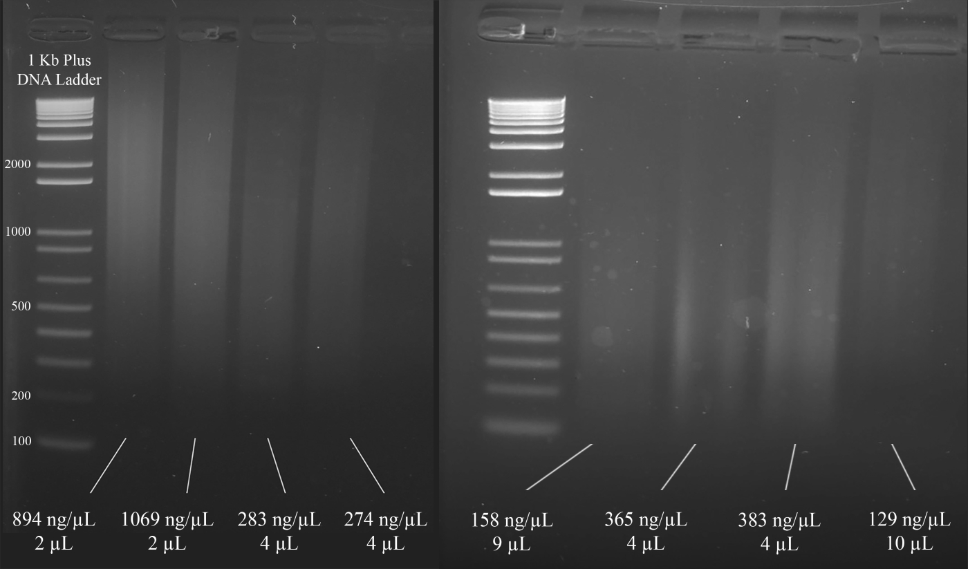
   3. Based on the results of steps 1.6.1 and 1.6.2, choose the volume of DNA to be used in the multiplex short tandem repeat (STR) polymerase chain reaction (PCR) amplification. Aim to use a minimum of 1000 ng of DNA in the PCR amplification that follows.
      NOTE: Figure 3 demonstrates representative examples of gels along with the concentrations of the DNA (based on the spectrophotometer results), and the volume of the DNA solution that is recommended for the multiplex STR PCR that follows.

Figure 3: Representative gel for DNA quantification. Included are the concentrations of each DNA, as measured using a spectrophotometer, and the quantities used for the multiplex PCR. Please click here to view a larger version of this figure.

7. PCR amplification
   1. Perform fluorescent microsatellite genotyping using a multiplex STR system (Table of Materials).
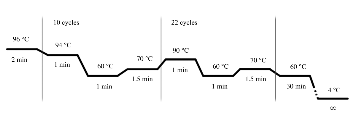
   2. Use the PCR conditions shown in Figure 4 for the PCR amplification using the multiplex STR system (Table of Materials).
      NOTE: The following primers are used in this multiplex STR system: D18S51, D21S11, TH01, D3S1358, Penta E, FGA, TPOX, D8S1179, vWA, Amelogenin, CSF1PO, D16S539, D7S820, D13S317, D5S818, and Penta D.

Figure 4: PCR cycle conditions for the multiplex STR system. Please click here to view a larger version of this figure.

8. Resolve the PCR products by capillary electrophoresis.
   1. Suspend 1 µL of each amplified sample in 0.5 µL of the multiplex system's internal standard lane and 9.5 µL of highly deionized formamide (Table of Materials).
   2. Run samples through a capillary electrophoresis instrument (Table of Materials) using an appropriate separation matrix (Table of Materials) for the instrument and the multiplex system's dye set.

9. Data analysis
   1. Analyze the data with a DNA fragment analysis software and compare the POC alleles to the parental alleles to determine their origin.
   2. Set up a size standard.
      NOTE: This allows the software to recognize the ladder that is used in the multiplex STR system, and to assign basepairs to the amplicons based on the ladder. The following steps are for one specific software (Table of Materials) but may be of help for setting up other types of software as well.
      1. Open the software. Click on Start New Project and then on New Size Standard.
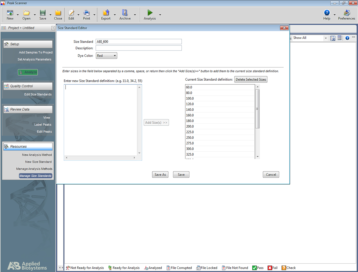
      2. Give the size standard a name (e.g., ABI_600).
      3. In the box named Enter New Size Standard definition: enter the following: 60, 80, 100, 120, 140, 160, 180, 200, 225, 250, 275, 300, 325, 350, 375, 400, 425, 450, 475, 500, 550, 600. Then click on Add Size(s).
         NOTE: The numbers entered will appear under the box on the right, which is named Current Size Standard Definition (see Figure 5).
      4. Click on Save.
   3. To import and analyze a file, click on Add Files, and choose the fsa file to be analyzed. Click on Add Selected Files and then on OK. Then follow these steps:
      1. Locate the Size Standard column and choose ABI_600 (or whichever name was given to the size standard).
      2. Under Analysis Method, click on Sizing Default - NPP and then click on the green Analyze button.
      3. The file is now ready for viewing. Adjust the viewing options to view the data as desired.
   4. Troubleshooting - analysis method
      NOTE: The software may sometimes fail to identify peaks and align them correctly. This happens when the peaks are either too low or too high. The following two analysis methods can correct for this and should be tried before a sample is retested.
      1. Analysis method 1 for high peaks:
         1. Click on New Analysis Method and name it High Peaks (or another name as per personal preference).
         2. Click on Range and then on Partial Range for the analysis and sizing. Then type in 100 for the Start Point and Start Size.
         3. For the Stop Point, enter 10,000. For the Stop Size, enter 1000.
         4. Then click on Minimum peak heights and change the numbers such that the peak threshold for the colors is as follows: Blue: 50; Green: 50; Yellow: 20; Red: 100; Orange: 5000.
         5. Save the new analysis method.
      2. Analysis method 2 for low peaks:
         1. Click on New Analysis Method and name it Low Peaks (or another name as per personal preference).
         2. Click on Range and then on Partial Range for the analysis and sizing. Then type in 100 for the Start Point and Start Size.
         3. For the Stop Point, enter 10,000. For the Stop Size, enter 1000.
         4. Then click on Quality Flags and change the Pass Range such that it reads From 0.5 to 1. Change the Low Quality Range such that it reads From 0.0 to 0.0. Change Assume Linearity to the following: from (bp) 100.0 to (bp) 800.0.
         5. Save the new analysis method.
            NOTE: It is now possible to reanalyze a file by choosing Low Peaks or High Peaks under Analysis Method and then clicking on the green Analyze button.

Figure 5: Screenshot showing the Size Standard Editor. Please click here to view a larger version of this figure.

2. Flow Cytometry

1. Choosing the ideal FFPE block
   1. Using H&E slides and a light microscope, select an FFPE block that has about 50−70% of its tissues composed of CV.
      NOTE: Figure 6 is a representative example of an appropriate block for flow cytometry analysis, as it is composed of roughly 50% CV (right half of the section) and 50% maternal tissues (left half). The presence of maternal tissues is important because they serve as an internal control for the diploid peak.
   2. For blocks that do not have the ideal amount of CV, enrich for CV as the sectioning is performed. To do so, identify which side of the freshly cut sections contains more CV according to its corresponding H&E slide. Based on that, use a blade to cut off the other half that needs to be discarded in order to enrich for CV.
      NOTE: Figure 7 shows a block that does not have sufficient CV for flow cytometry analysis. For blocks such as this one, the sections need to be cut such that the half that contains less CV gets discarded in order to increase the amounts of CV with respect to maternal tissues, as shown in the figure. Be sure to cut more sections to compensate for what is discarded.

Figure 6: H&E section representing a POC block that is ideal for flow cytometry. Please click here to view a larger version of this figure.

Figure 7: H&E section representing a more difficult block for flow cytometry. This representative H&E section shows that only the bottom half of this section should be used for flow cytometry analysis, with the goal of enriching for the CV. The outlined area, labelled "CV," is mostly made up of CV. Please click here to view a larger version of this figure.

2. Sectioning
   1. Leave the blocks on ice for 15 min to facilitate the sectioning.
   2. Using the best possible FFPE block, cut four sections that are 50 µm thick (or two 100 µm thick sections) using a microtome.
      NOTE: For flow cytometry it is preferable to have thicker sections.
   3. In the case that an ideal FFPE block is not available, aim to maintain the ratio of CV to maternal tissue nonetheless. For example, if only 30% of the block is made up of CV while the rest has maternal tissues, then remove at least half of the section that contains the maternal tissues and use more sections to compensate (see Figure 7).
   4. Place the sections in labelled 15 mL tubes.
      NOTE: Be sure to tape over the labels because the organic reagents used in the next step can dissolve and remove ink.
3. Flow cytometry protocol from FFPE tissues
   1. Deparaffinization and rehydration 
      1. Perform the following washes (Table 3) under a fume hood. 
      2. Fill the 15 mL tube with 6 mL of the appropriate reagent, following the order presented in Table 3, leave the sections in the reagents for the respective duration, and then remove the reagent using vacuum suction and a glass Pasteur pipette. 
      3. Between each step, dip the Pasteur pipette first in 70% ethanol, then in distilled water, and then proceed to the next step.
      4. Be very careful not to remove pieces of tissue along with the reagent. Tilt the 15 mL tube to a 60-degree angle to facilitate suction of the liquid reagent without drawing tissues. 
         CAUTION: The discarded liquids contain xylene and should be disposed of in xylene waste containers.
   2. Solution preparation
      1. Prepare citrate solution by dissolving 2 g of citric acid in 1 L of double distilled water. Bring the pH to 6. Store at 4 °C.
      2. Prepare pepsin solution by dissolving 0.01 g of pepsin in 2 mL of 9 parts per thousand NaCl, pH 1.64. This is for one sample.
         CAUTION: Pepsin is toxic and can easily disperse and become airborne. Wear a mask when handling pepsin in its powder form and wipe down all of the working area after using it.
      3. Propidium Iodide (PI)-ribonuclease A solution preparation for one sample.
         1. Mix 50 µL of PI with 450 µL of PBS (to dilute 10x).
         2. Add 50 µL of ribonuclease A (1 mg/mL) to the mixture. Keep wrapped in foil at all times.
   3. Digestion and staining
      1. Add 4 °C citrate solution to the 15 mL tubes then place in an 80 °C water bath for 2 h.
      2. Let the solution cool down to room temperature (15 min). Remove the citrate solution.
      3. Add 6 mL of 1x PBS, vortex, and wait 1−2 min to allow the tissues to settle to the bottom. Remove the 1x PBS using vacuum suction and a glass Pasteur pipette.
      4. Add 1 mL of pepsin solution (preheated to 37 °C) and place in a 37 °C dry bath for 30 min. Vortex every 10 min. Prepare the PI-ribonuclease A solution in the last 10 min of this incubation.
      5. Add 6 mL of 1x PBS, vortex, and wait 1−2 min to allow the tissues to settle to the bottom. Remove the 1x PBS using vacuum suction and a glass Pasteur pipette.
      6. Add 550 µL of the PI-ribonuclease A solution and place the samples in a 37 °C dry bath for 30 min.
         NOTE: At this point, the samples can be wrapped in foil and left overnight at 4 °C till the next morning.
      7. Filter the solution through a 48-µm filtration mesh. Collect the filtrate in polystyrene round-bottom tubes, which can be used with the flow cytometer. Use forceps to place a 5 cm by 5 cm piece of filtration mesh in the top part of the tube, such that the liquid can be pipetted through the mesh and into the tube. 
         NOTE: The samples are now ready to be run with the flow cytometer. Keep them wrapped in foil until they are ready to be run.
   4. Run samples with a flow cytometer with the help of the organization’s flow cytometry platform technician.
      NOTE: The PE channel is used to detect the PI-stained DNA and the flow rate should be set to Slow during acquisition. Ensure that the voltage is chosen such that the diploid peak is roughly at 200 along the PE-A x-axis to facilitate analysis and interpretation. Aim to record a minimum of 20,000 events per sample.  

Reagent used (6 mL each)	Duration
1) Xylene	2 x 10 min
2) 100% Ethanol	2 x 10 min
3) 95% Ethanol	10 min
4) 70% Ethanol	10 min
5) 50% Ethanol	10 min
6) Distilled water	2 x 10 min

Table 3: Reagents and durations for deparaffinization and rehydration.

4. Flow cytometry data analysis
   1. Analyze data with a flow cytometry analysis software (Table of Materials).
      NOTE: The following steps are for one specific software (Table of Materials) but may be of help for setting up other types of software as well.
      1. After running the samples on a flow cytometer, download FCS 2.0 files for analysis.
      2. Open the flow cytometry analysis software, click on File | New Document.
      3. Click on the Histogram icon (), and then drag the pointer to make a rectangle.
      4. Browse for the FCS file and then click on Open. Along the x-axis, click on FCS-A and then select PE-A.
      5. Click on the Dot Plot icon () and then drag the pointer to create another rectangle beneath the histogram plot. Then browse for the same FCS file that was selected for the histogram.
      6. Change the x-axis of the dot plot to PE-A and the y-axis to PE-W.
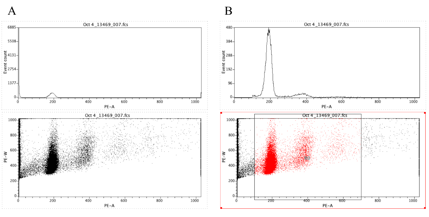
         NOTE: Figure 8A demonstrates the appearance of the plots at this point.
      7. Click on the Region icon () and draw a box on the dot plot that starts before the diploid peak (around 100 on the x-axis in Figure 8B) and that ends around 700 on the x-axis, as shown in the dot plot in Figure 8B.
         NOTE: The diploid peak in Figure 8 is roughly at 200 on the x-axis. This is chosen arbitrarily as the samples are recorded through the flow cytometer, simply to facilitate analysis and interpretation of the results.
      8. Click on Plot | Edit Regions/Gates, then type R0 in the cell that is next to the G0 cell under Strategy. Then click on Close.
      9. Click anywhere on the histogram, then on Plot | Format Plot/Overlay. Under Gate, select G0 = R0 and then click on OK.
         NOTE: This is the gating step that allows one to better visualize the ploidy peaks. The histogram should now look like the histogram in Figure 8B. It is possible to play around with the gate created (by moving the box drawn in step 2.4.1.7) in order to focus on specific regions of the dot plot.
      10. To label the plots, click on the Text Area icon (), then drag the pointer to create a box at the top of the document, and then type in the following information: Patient ID, POC ID and the block used (since there may be several blocks for one POC), percent CV present on the block, voltage used to run the sample, and the date.

Figure 8: Screenshot displaying a histogram and a dot plot of a representative sample that is ungated (A) and gated (B). Please click here to view a larger version of this figure.

Results

The complexity of molar tissues and the fact that they may have various genotypes necessitates stringent analysis and the use of several methods such as morphological evaluation, p57 immunohistochemistry, microsatellite genotyping, flow cytometry, and FISH. For example, one patient (1790) was referred with two PHM that were found to be triploid by microarray analysis of the POCs only. The patient was therefore diagnosed with recurrent PHM. Microsatellite genotyping of her two "PHM"...

Discussion

HM are abnormal human pregnancies with heterogeneous etiologies and have different histological and genotypic types, which makes their accurate classification and diagnosis challenging. Histopathological morphological evaluation was often proven inaccurate and is therefore unreliable on its own to classify HM into CHM and PHM and distinguish them from non-molar miscarriages. Therefore, an accurate diagnosis of HM requires the use of other methods such as multiplex microsatellite DNA genotyping, ploidy analysis by flow cy...

Materials

Name	Company	Catalog Number	Comments
BD FACS Canto II	BD BioSciences	338960
Capillary electrophoresis instrument: Genomes Applied Biosystems 3730xl DNA Analyzer	Applied biosystems	313001R	Service offered by the Centre for Applied Genomics (http://www.tcag.ca)
Citric acid	Sigma	251275
Cytoseal 60, histopathology mounting medium	Fisher	23244257
Eosin Y stock solution (1%)	Fisher	SE23-500D
FCSalyzer - flow cytometry analysis software	SourceForge	-	https://sourceforge.net/projects/fcsalyzer/
FFPE Qiagen kit	Qiagen	80234
Forceps	Fine Science Tools	11295-51	For sectioning and for the cleaning process
Glacial Acetic Acid (Concentrated)	Sigma	A6283-500mL
Glass coverslips: Cover Glass	Fisher	12-541a
Hematoxylin	Fisher	CS401-1D
Highly deionized formamide: Hi-Di Formamide	Thermofisher	4311320
IHC platform: Benchmark Ultra	Roche	-
Kimwipes	Ultident	30-34120
Microtome	Leica	RM2135
Microtome blades	Fisher	12-634-1C
Nitex filtering mesh, 48 microns	Filmar	74011	http://www.filmar.qc.ca/index.php?filet=produits&id=51&lang=en ; any other filter is suitable, but this is an inexpensive and effective option from a non-research company
p57 antibody	Cell Marque	457M
Pasteur pipette	VWR	53499-632
PCR machine	Perkin Elmer, Applied Biosystems	GeneAmp PCR System 9700
PeakScanner 1.0	Applied Biosystems	4381867	Software for genotyping analysis.
Pepsin from porcine gastric mucosa	Sigma	P7012
Polystyrene round-bottom tubes	BD Falcon	352058
Positively charged slides: Superfrost Plus 25x75mm	Fisher	1255015
PowerPlex 16 HS System	Promega Corporation	DC2102
Propidium Iodide	Sigma	P4864
Ribonuclease A from bovine pancreas	Sigma	R4875
Separation matrix: POP-7 Polymer	Thermofisher	4352759
UltraPure Agarose	Fisher	16500-500
Xylene	Fisher	X3P1GAL

References

- Szulman, A. E., Surti, U. The syndromes of hydatidiform mole. II. Morphologic evolution of the complete and partial mole. American Journal of Obstetrics & Gynecology. 132 (1), 20-27 (1978).
- Fukunaga, M., et al. Interobserver and intraobserver variability in the diagnosis of hydatidiform mole. The American Journal of Surgical Pathology. 29 (7), 942-947 (2005).
- Gupta, M., et al. Diagnostic reproducibility of hydatidiform moles: ancillary techniques (p57 immunohistochemistry and molecular genotyping) improve morphologic diagnosis for both recently trained and experienced gynecologic pathologists. The American Journal of Surgical Pathology. 36 (12), 1747-1760 (2012).
- Howat, A. J., et al. Can histopathologists reliably diagnose molar pregnancy?. Journal of Clinical Pathology. 46 (7), 599-602 (1993).
- Banet, N., et al. Characteristics of hydatidiform moles: analysis of a prospective series with p57 immunohistochemistry and molecular genotyping. Modern Pathology. 27 (2), 238-254 (2014).
- Lipata, F., et al. Precise DNA genotyping diagnosis of hydatidiform mole. Obstetrics & Gynecology. 115 (4), 784-794 (2010).
- Buza, N., Hui, P. Partial hydatidiform mole: histologic parameters in correlation with DNA genotyping. International Journal of Gynecologic Pathology. 32 (3), 307-315 (2013).
- Fisher, R. A., et al. Frequency of heterozygous complete hydatidiform moles, estimated by locus-specific minisatellite and Y chromosome-specific probes. Human Genetics. 82 (3), 259-263 (1989).
- Murdoch, S., et al. Mutations in NALP7 cause recurrent hydatidiform moles and reproductive wastage in humans. Nature Genetics. 38 (3), 300-302 (2006).
- Parry, D. A., et al. Mutations causing familial biparental hydatidiform mole implicate c6orf221 as a possible regulator of genomic imprinting in the human oocyte. American Journal of Human Genetics. 89 (3), 451-458 (2011).
- Nguyen, N. M., Slim, R. Genetics and Epigenetics of Recurrent Hydatidiform Moles: Basic Science and Genetic Counselling. Current Obstetrics and Gynecology Reports. 3, 55-64 (2014).
- Sebire, N. J., Savage, P. M., Seckl, M. J., Fisher, R. A. Histopathological features of biparental complete hydatidiform moles in women with NLRP7 mutations. Placenta. 34 (1), 50-56 (2013).
- Nguyen, N. M., et al. Comprehensive genotype-phenotype correlations between NLRP7 mutations and the balance between embryonic tissue differentiation and trophoblastic proliferation. Journal of Medical Genetics. 51 (9), 623-634 (2014).
- Brown, L., et al. Recurrent pregnancy loss in a woman with NLRP7 mutation: not all molar pregnancies can be easily classified as either "partial" or "complete" hydatidiform moles. International Journal of Gynecologic Pathology. 32 (4), 399-405 (2013).
- Colgan, T. J., Chang, M. C., Nanji, S., Kolomietz, E. A Reappraisal of the Incidence of Placental Hydatidiform Mole Using Selective Molecular Genotyping. The International Journal of Gynecological Cancer. 26 (7), 1345-1350 (2016).
- Murphy, K. M., McConnell, T. G., Hafez, M. J., Vang, R., Ronnett, B. M. Molecular genotyping of hydatidiform moles: analytic validation of a multiplex short tandem repeat assay. The Journal of Molecular Diagnostics. 11 (6), 598-605 (2009).
Reprints and Permissions
Request permission to reuse the text or figures of this JoVE article
Request PermissionThis article has been published
Video Coming Soon
Copyright © 2025 MyJoVE Corporation. All rights reserved