Method Article
Cryo-EM and Single-Particle Analysis with Scipion
In This Article
Summary
Single-particle analysis in cryo-electron microscopy is one of the main techniques used to determine the structure of biological ensembles at high resolution. Scipion provides the tools to create the whole pipeline to process the information acquired by the microscope and achieve a 3D reconstruction of the biological specimen.
Abstract
Cryo-electron microscopy has become one of the most important tools in biological research to reveal the structural information of macromolecules at near-atomic resolution. In single-particle analysis, the vitrified sample is imaged by an electron beam and the detectors at the end of the microscope column produce movies of that sample. These movies contain thousands of images of identical particles in random orientations. The data need to go through an image processing workflow with multiple steps to obtain the final 3D reconstructed volume. The goal of the image processing workflow is to identify the acquisition parameters to be able to reconstruct the specimen under study. Scipion provides all the tools to create this workflow using several image processing packages in an integrative framework, also allowing the traceability of the results. In this article the whole image processing workflow in Scipion is presented and discussed with data coming from a real test case, giving all the details necessary to go from the movies obtained by the microscope to a high resolution final 3D reconstruction. Also, the power of using consensus tools that allow combining methods, and confirming results along every step of the workflow, improving the accuracy of the obtained results, is discussed.
Introduction
In cryo-electron microscopy (cryo-EM), single particle analysis (SPA) of vitrified frozen-hydrated specimens is one of the most widely used and successful variants of imaging for biological macromolecules, as it allows to understand molecular interactions and the function of biological ensembles1. This is thanks to the recent advances in this imaging technique that gave rise to the "resolution revolution"2 and have allowed the successful determination of biological 3D structures with near-atomic resolution. Currently, the highest resolution achieved in SPA cryo-EM was 1.15 Å for apoferritin3 (EMDB entry: 11668). These technological advances comprise improvements in the sample preparation4, the image acquisition5, and the image processing methods6. This article is focused on this last point.
Briefly, the goal of the image processing methods is to identify all the acquisition parameters to invert the imaging process of the microscope and recover the 3D structure of the biological specimen under study. These parameters are the gain of the camera, the beam-induced movement, the aberrations of the microscope (mainly the defocus), the 3D angular orientation and translation of each particle, and the conformational state in case of having a specimen with conformational changes. However, the number of parameters is very high and cryo-EM requires using low-dose images to avoid radiation damage, which significantly reduces the Signal-to-Noise Ratio (SNR) of the acquired images. Thus, the problem cannot be unequivocally solved and all the parameters to be calculated only can be estimations. Along the image processing workflow, the correct parameters should be identified, discarding the remaining ones to finally obtain a high-resolution 3D reconstruction.
The data generated by the microscope are gathered in frames. Simplifying, a frame contains the number of electrons that have arrived at a particular position (pixel) in the image, whenever electron-counting detectors are used. In a particular field of view, several frames are collected and this is called a movie. As low electron doses are used to avoid radiation damage that could destroy the sample, the SNR is very low and the frames corresponding to the same movie need to be averaged to obtain an image revealing structural information about the sample. However, not only a simple average is applied, the sample can suffer shifts and other kinds of movements during the imaging time due to the beam-induced movement that need to be compensated. The shift-compensated and averaged frames originate a micrograph.
Once the micrographs are obtained, we need to estimate the aberrations introduced by the microscope for each of them, called Contrast Transfer Function (CTF), which represents the changes in the contrast of the micrograph as a function of frequency. Then, the particles can be selected and extracted, which is called particle picking. Every particle should be a small image containing only one copy of the specimen under study. There are three families of algorithms for particle picking: 1) the ones that only use some basic parameterization of the appearance of the particle to find them in the whole set of micrographs (e.g., particle size), 2) the ones that learn how the particles look like from the user or a pretrained set, and 3) the ones that use image templates. Each family has different properties that will be shown later.
The extracted set of particles found in the micrographs will be used in a 2D classification process that has two goals: 1) cleaning the set of particles by discarding the subset containing pure noise images, overlapping particles, or other artifacts, and 2) the averaged particles representing each class could be used as initial information to calculate a 3D initial volume.
The 3D initial volume calculation is the next crucial step. The problem of obtaining the 3D structure can be seen as an optimization problem in a multidimensional solution landscape, where the global minimum is the best 3D volume that represents the original structure, but several local minima representing suboptimal solutions can be found, and where it is very easy to get trapped. The initial volume represents the starting point for the searching process, so bad initial volume estimation could prevent us to find the global minimum. From the initial volume, a 3D classification step will help to discover different conformational states and to clean again the set of particles; the goal is to obtain a structurally homogeneous population of particles. After that, a 3D refinement step will be in charge of refining the angular and translation parameters for every particle to get the best 3D volume possible.
Finally, in the last steps, the obtained 3D reconstruction can be sharpened and polished. Sharpening is a process of boosting the high frequencies of the reconstructed volume, and the polishing is a step to further refine some parameters, as CTF or beam-induced movement compensation, at the level of particles. Also, some validation procedures could be used to better understand the achieved resolution at the end of the workflow.
After all these steps, the tracing and docking processes7 will help to give a biological meaning to the obtained 3D reconstruction, by building atomic models de novo or fitting existing models. If high resolution is achieved, these processes will tell us the positions of the biological structures, even of the different atoms, in our structure.
Scipion8 allows creating the whole workflow combining the most relevant image processing packages in an integrative way. Xmipp9, Relion10, CryoSPARC11, Eman12, Spider13, Cryolo14, Ctffind15, CCP416, Phenix17, and many more packages can be included in Scipion. Also, it incorporates all the necessary tools to benefit the integration, interoperability, traceability, and reproducibility to make a full tracking of the entire image-processing workflow8.
One of the most powerful tools that Scipion allows us to use is the consensus, which means to compare the results obtained with several methods in one step of the processing, making a combination of the information conveyed by different methods to generate a more accurate output. This could help to boost the performance and improve the achieved quality in the estimated parameters. Note that a simpler workflow can be build without the use of consensus methods; however, we have seen the power of this tool22,25 and the workflow presented in this manuscript will use it in several steps.
All the steps that have been summarized in the previous paragraphs will be explained in detail in the following section and combined in a complete workflow using Scipion. Also, how to use the consensus tools to achieve a higher agreement in the generated outputs will be shown. To that end, the example dataset of the Plasmodium falciparum 80S Ribosome has been chosen (EMPIAR entry: 10028, EMDB entry: 2660). The dataset is formed by 600 movies of 16 frames of size 4096x4096 pixels at a pixel size of 1.34Å taken at an FEI POLARA 300 with an FEI FALCON II camera, with a reported resolution at EMDB is 3.2Å18 .
Protocol
1. Creating a project in Scipion and importing the data
- Open Scipion and click on Create Project, specify the name for the project and the location where it will be saved (Supplemental Figure 1). Scipion will open the project window showing a canvas with, on the left side, a panel with a list of available methods, each of them represents one image processing tool that can be used to manage data.
NOTE: Ctrl+F can be used to find a method if it does not appear in the list. - To import the movies taken by the microscope select the pwem - import movies on the left panel (or type it when pressing Ctrl+F).
- A new window will be opened (Supplemental Figure 2). There, include the path to the data, and the acquisition parameters. In this example, use the following setup: Microscope voltage 300 kV, Spherical aberration 2.0 mm, Amplitude Contrast 0.1, Magnification rate 50000, Sampling rate mode to From image, and Pixel size 1.34 Å. When all the parameters in the form are filled, click on the Execute button.
NOTE: When a method starts, a box appears in the canvas in yellow color labeled as running. When a method finishes, the box changes to green, and the label changes to finished. In case of an error during the execution of a method, the box will appear in red, labeled as failed. In that case, check the bottom part of the canvas, in the Output Log tab an explanation of the error will appear. - When the method finishes, check the results in the bottom part of the canvas in the Summary tab. Here, the outputs generated by the method are presented, in this case, the set of movies. Click on Analyze Results button and a new window will appear with the list of movies.
2. Movie alignment: from movies to micrographs
- Use the method xmipp3 - optical alignment which implements Optical flow19. Use the following parameters to fill in the form (Supplemental Figure 3): the Input Movies are those obtained in step 1, the range in Frames to ALIGN is from 2 to 13, the other options stay with the default values. Execute the program.
NOTE: The parameters in bold in a form must be always filled. The others will have a default value or will not be obligatorily required. In the upper part of the form window, the fields where the computational resources are distributed can be found, as threads, MPIs, or GPUs. - Click on Analyze Results to check the obtained micrographs and the trajectory of the estimated shifts (Figure 1). For every micrograph seen: look at the power spectral density (PSD), the trajectories obtained to align the movie (one point per frame) in cartesian and polar coordinates, and the file name of the obtained micrograph (clicking on it, the micrograph can be inspected). Notice that the particles of the specimen are much more visible in the micrograph, as compared to a single frame of the movie.
3. CTF estimation: calculating the aberrations of the microscope
- First, use the method grigoriefflab - ctffind15. The setup is: the Input Micrographs are the output of step 2, the Manual CTF Downsampling factor is set to 1.5, and the Resolution range goes from 0.06 to 0.42. Moreover, in the Advanced options (that can be found by selecting this choice in the Expert Level of the form), set the Window size to 256. The remaining parameters stay with the default values (Supplemental Figure 4).
NOTE: In most of the methods in Scipion the Advanced option shows more configuration parameters. Use these options carefully, when the program to be launched is completely known and the meaning of the parameters is understood. Some parameters can be difficult to fill without having a look at the data; in that case, Scipion shows a magic wand on the right side that will show a wizard window (Supplemental Figure 5). For example, in the Resolution field of this form is especially useful, as these values should be selected to approximately cover the region from the first zero to the last noticeable ring of the PSD. - Click on Execute and on Analyze Results (Figure 2) when the method finishes. Check that the estimated CTF matches with the experimental one. To that end, look at the PSD and compare the estimated rings in the corner with the ones coming from the data. Also check the obtained defocus values to find any unexpected values and respective micrographs can be discarded or recalculated. In this example, the whole set of micrographs can be used.
NOTE: Use the buttons in the bottom part of the window to make a subset of micrographs (with Micrographs red button) and to recalculate a CTF (with Recalculate CTFs red button), in case of needing. - To refine the previous estimation, use xmipp3 - ctf estimation20. Select as Input Micrographs the output of step 2, select the option Use defoci from a previous CTF estimation, as Previous CTF estimation choose the output of grigoriefflab - ctffind, and, in the Advanced level, change the Window size to 256 (Supplemental Figure 6). Run it.
- Click on Analyze Results to check the obtained CTFs. With this method, more data is estimated and represented in some extra columns. As none of them show incorrect estimated values, all the micrographs will be used in the following steps.
4. Particle picking: finding particles in the micrographs
- Before starting the picking, carry out a preprocess of the micrographs. Open xmipp3 - preprocess micrographs, set as Input micrographs those obtained in step 2 and select the options Remove bad pixels? with Multiple of Stddev to 5, and Downsample micrographs? with a Downsampling factor of 2 (Supplemental Figure 7). Click on Execute and check that the size of the resulting micrographs has been reduced.
- For the picking use xmipp3 - manual-picking (step 1) and xmipp3 - auto-picking (step 2)21. The manual picking allows to manually prepare a set of particles with which the auto-picking step will learn and generate the complete set of particles. First, run xmipp3 - manual-picking (step 1) with Input Micrographs as the micrographs obtained in the previous preprocess. Click on Execute and a new interactive window will appear (Figure 3).
- In this window a list of the micrographs (Figure 3a) and other options is presented. Change Size (px) to 150, this will be the size of the box containing each particle. The selected micrograph appears in a bigger window. Choose a region and pick all the visible particles in it (Figure 3b). Then, click on Activate Training to start the learning. The remaining regions of the micrograph are automatically picked (Figure 3c). Check the picked particles and include more by clicking on it, or remove the incorrect ones with shift+clicking, if necessary.
- Select the next micrograph in the first window. The micrograph will be automatically picked. Check again to include or remove some particles, if necessary. Repeat this step with, approximately, 5 micrographs to create a representative training set.
- Once this is done, click on Coordinates in the main window to save the coordinates of all the picked particles. The training set of particles is ready to go to the auto picking to complete the process for all micrographs.
- Open xmipp3 - auto-picking (step 2) indicating in Xmipp particle picking run the previous manual picking, and Micrographs to pick as Same as supervised. Click on Execute. This method will generate as output a set of around 100000 coordinates.
- Apply a consensus approach, so carry out a second picking method to select the particles in which both methods agree. Open sphire - cryolo picking14 and select the preprocessed micrographs as Input Micrographs, Use general model? to Yes, with a Confidence threshold of 0.3, and a Box Size of 150 (Supplemental Figure 8). Run it. This method should generate also around 100000 coordinates.
- Run xmipp3 - deep consensus picking22. As Input coordinates include the output of sphire - cryolo picking (step 4.7) and xmipp3 - auto-picking (step 4.6), set Select model type to Pretrained, and Skip training and score directly with pretrained model? To Yes (Supplemental Figure 9). Run it.
- Click on Analyze Results and, in the new window, on the eye icon next to Select particles/coordinates with high 'zScoreDeepLearning1' values. A new window will be opened with a list of all particles (Figure 4). The zScore values in the column give an insight into the quality of a particle, low values mean bad quality.
- Click on the label_xmipp_zScoreDeepLearning to order the particles from highest to lowest zScore. Select the particles with zScore higher than 0.75 and click on Coordinates to create the new subset. This should create a subset with approximately 50000 coordinates.
- Open xmipp3 - deep micrograph cleaner. Select as Input coordinates the subset obtained in the previous step, Micrographs source as same as coordinates, and keep Threshold at 0.75. Run it. Check in the Summary tab that the number of coordinates has been reduced, although in this case, only few coordinates are removed.
NOTE: This step is able to additionally clean the set of coordinates and could be very useful in cleaning other datasets with more movie artifacts as carbon zones or large impurities. - Run xmipp3 - extract particles (Supplemental Figure 10). Indicate as Input coordinates the coordinates obtained after the previous step, Micrographs source as other, Input micrographs as the output of step 2, CTF estimation as the output of the xmipp3 - ctf estimation, Downsampling factor to 3, and Particle box size to 100. In the Preprocess tab of the form select Yes to all. Run it.
- Check that the output should contain the particles in reduced size of 100x100 pixels and a pixel size of 4.02Å/px.
- Run again xmipp3 - extract particles changing the following parameters: Downsampling factor to 1, and Particle box size to 300. Check that the output is the same set of particles but now at the full resolution.
5. 2D classification: grouping similar particles together
- Open the method cryosparc2 - 2d classification11 with Input particles as those obtained in step 4.11 and, in the 2D Classification tab, the Number of classes to 128, keep all the other parameters with the default values. Run it.
- Click on Analyze Results and then on the eye icon next to Display particle classes with Scipion (Figure 5). This classification will help to clean the set of particles, as several classes will appear noisy or with artifacts. Select the classes containing good views. Click on Particles (red button in the lower part of the window) to create the cleaner subset.
- Now, open xmipp3 - cl2d23 and set as Input images the images obtained in the previous step and Number of classes as 128. Click on Execute.
NOTE: This second classification is used as additional cleaning step of the set of particles. Usually is useful to remove as much noisy particles as it is possible. However, if a simpler workflow is desired, only one 2D classification method can be used. - When the method finishes, check the 128 generated classes by clicking on Analyze Results and on What to show: classes. Most of the generated classes show a projection of the macromolecule with some level of detail. However, some of them appear noisy (in this example approximately 10 classes). Select all the good classes and click on the Classes button to generate a new subset with only the good ones. This subset will be used as input to one of the methods to generate an initial volume. With the same selected classes click on Particles to create a cleaner subset after removing those belonging to the bad classes.
- Open pwem - subset with Full set of items as the output of 4.13 (all particles at the full size), Make random subset to No, Other set as the subset of particles created in the previous step, and Set operation as intersection. This will extract the previous subset from the particles at full resolution.
6. Initial volume estimation: building the first guess of the 3D volume
- In this step, estimate two initial volumes with different methods and then use a consensus tool to generate the final estimated 3D volume. Open xmipp3 - reconstruct significant24 method with Input classes as those obtained after step 5, Symmetry group as c1, and keep the remaining parameters with their default values (Supplemental Figure 11). Execute it.
- Click on Analyze Results. Check that a low resolution volume of size 100x100x100 pixels and a pixel size of 4.02Å/px is obtained.
- Open xmipp3 - crop/resize volumes (Supplemental Figure 12) using as Input Volumes the one obtained in the previous step, Resize volumes? to Yes, Resize option to Sampling Rate, and Resize sampling rate to 1.34 Å/px. Run it. Check in the Summary tab that the output volume has the correct size.
- Now, create the second initial volume. Open relion - 3D initial model10, as Input particles use the good particles at full resolution (output of 5.5) and set Particle mask diameter to 402Å, keep the remaining parameters with the default values. Run it.
- Click on Analyze Results and then in Display volume with: slices. Check that a low resolution volume but with the main shape of the structure is obtained (Supplemental Figure 13).
- Now, open pwem - join sets to combine the two generated initial volumes to create the input to the consensus method. Just indicate Volumes as Input type and select the two initial volumes in Input set. Run it. The output should be a set containing two items with both volumes.
- The consensus tool is the one included in xmipp3 - swarm consensus25. Open it. Use as Full-size Images the good particles at full resolution (output of 5.5), as Initial volumes the set with two items generated in the previous step, and be sure that Symmetry group is c1. Click on Execute.
- Click on Analyze Results. Check that a more detailed output volume is obtained (Figure 6). Although there is more noise surrounding the structure, to have more details in the structure map will help the following refinement steps to avoid local minima.
NOTE: If UCSF Chimera26 is available, use the last icon in the upper part of the window to make a 3D visualization of the obtained volume. - Open and execute relion - 3D auto-refine10 to make a first 3D angular assignment of the particles. Select as Input particles the output of 5.5, and set Particle mask diameter to 402Å. In Reference 3D map tab, select as Input volume the one obtained in the previous step, Symmetry as c1, and Initial low-pass filter to 30Å (Supplemental Figure 14).
- Click on Analyze Results. In the new window select final as Volume to visualize and click on Display volume with: slices to see the obtained volume. Check also the Fourier shell correlation (FSC) by clicking on Display resolution plots in the results window and the angular coverage in Display angular distribution: 2D plot (Figure 7). The reconstructed volume contains much more details (probably with some blurred areas in the outer part of the structure), and the FSC crosses the threshold of 0.143 around 4.5Å. The angular coverage covers the whole 3D sphere.
7. 3D classification: discovering conformational states
- Using a consensus approach, if different conformational states are in the data can be discovered. Open relion - 3D classification10 (Supplemental Figure 15). As Input particles use those just obtained in 6.10, and set Particle mask diameter to 402Å. In the Reference 3D map tab, use as Input volume the one obtained after step 6.10, set Symmetry to c1, and Initial low-pass filter to 15Å. Finally, in Optimization tab, set the Number of classes to 3. Run it.
- Check the results by clicking on Analyze Results, select Show classification in Scipion. The three generated classes and some interesting measures are shown. The first two classes should have a similar number of assigned images (size column) and look very similar, whilst the third one has fewer images and a more blurred appearance. Also, the rlnAccuracyRotations and rlnAccuracyTranslations should be clearly better for the first two classes. Select the two best classes and click on the Classes button to generate a subset containing them.
- Repeat steps 7.1 and 7.2 to generate a second group of good classes. Both will be the input of the consensus tool.
- Open and run xmipp3 - consensus classes 3D and select as Input Classes the two subsets generated in the previous steps.
- Click on Analyze Results. The number of coincident particles between classes is presented: the first value is the number of coincident particles in the first class of subset 1 and the first class of subset 2, the second value is the number of coincident particles in the first class of subset 1 and the second class of subset 2, etc. Check that the particles are randomly assigned to classes one or two, which means that the 3D classification method is not able to find conformational changes. Given this result, the whole set of particles will be used to continue processing.
8. 3D refinement: refining angular assignments of a homogeneous population
- Again, apply a consensus approach in this step. First, open and run pwem - subset with Full set of items as the output of 6.9, Make random subset to Yes, and Number of elements to 5000. With this, a subset of images with a previous alignment to train the method used in the following step is created.
- Open xmipp3 - deep align, set Input images as the output of good particles obtained in 5.5, Volume as the one obtained after 6.10, Input training set as the one created in the previous step, Target resolution to 10Å, and keep the remaining parameters with the default values (Supplemental Figure 16). Click on Execute.
- Click on Analyze Results to check the obtained angular distribution, where there are no missing directions and the angular coverage slightly improves compared to the one of 6.10 (Figure 8).
- Open and execute xmipp3 - compare angles and select as Input particles 1 the output of 6.9 and Input particles 2 the output of 8.2, make sure that the Symmetry group is c1. This method calculates the agreement between xmipp3 - deep align and relion - 3D auto refine.
- Click on Analyze Results, the list of particles, with the obtained differences in shifts and angles, is shown. Click on the bar icon in the upper part of the window, another window will be opened that allows making plots of the calculated variables. Select _xmipp_angleDiff and click on Plot to see a representation of the angular differences per particle. Do the same with _xmipp_shiftDiff. In these figures, approximately in half of the particles both methods agree (Figure 9). Select the particles with angular differences lower than 10º and create a new subset.
- Now, open xmipp3 - highres27 to make a local refinement of the assigned angles. First, select as Full-size Images the images obtained in the previous step, and as Initial volumes the output of 6.9, set Radius of particle to 150 pixels, and Symmetry group as c1. In the Angular assignment tab, set the Image alignment to Local, Number of iterations to 1, and Max. Target Resolution as 5Å/px (Supplemental Figure 17). Run it.
- In the Summary tab check that the output volume is smaller than 300x300x300 pixels and with slightly higher pixel size.
- Click on Analyze Results to see the obtained results. Click on Display resolution plots to see the FSC, and on Display volume: Reconstructed to see the obtained volume (Supplemental Figure 18). A good resolution volume close to 4-3.5Å is obtained.
- Click on Display output particles and, in the window with the list of particles, click on the bar icon. In the new window, select Type as Histogram, with 100 Bins, select _xmipp_cost label, and finally press Plot (Supplemental Figure 19). This way, the histogram of the cost label is presented, which contains the correlation of the particle with the projection direction selected for it. In this case, a unimodal density function is obtained, which is a sign of not having different populations in the set of particles. Thus all of them will be used to continue the refinement
NOTE: In case of seeing a multimodal density function, the set of particles belonging to the higher maximum should be selected to continue the workflow only with them. - Open and execute again xmipp3 - highres with Continue from a previous run? to Yes, set as Full-size Images those obtained after 8.5, and Select previous run with the previous execution of Xmipp Highres. In the Angular assignment tab, set the Image alignment to Local, with 1 iteration and 2.6Å/px as target resolution (full resolution).
- Now the output should contain a volume at full resolution (size 300x300x300 pixels). Click on Analyze Results to check again the obtained volume and the FSC, which now should be a high resolution volume at around 3Å (Figure 10).
9. Evaluation and post-processing
- Open xmipp3 - local MonoRes28. This method will calculate the resolution locally. Set as Input Volume the one obtained after 8.10, set Would you like to use half volumes? to Yes, and Resolution Range from 1 to 10Å. Run it.
- Click on Analyze Results and select Show resolution histogram and Show colored slices (Figure 11). The resolution in the different parts of the volume is shown. Most of the voxels of the central part of the structure should present resolutions around 3Å, whilst the worst resolutions are achieved in the outer parts. Also, a histogram of the resolutions per voxel is shown with a peak around (even below) 3Å.
- Open and run xmipp3 - localdeblur sharpening29 to apply a sharpening. Select as Input Map the one obtained in 8.10, and as Resolution Map the one obtained in the previous step with MonoRes.
- Click on Analyze Results to check the obtained volumes. Open the last one, corresponding to the last iteration of the algorithm. It is recommend opening the volume with other tools, such as UCSF Chimera26, to see better the features of the volume in 3D (Figure 12).
- Finally, open the validation tool included in xmipp3 - validate overfitting30 that will show how the resolution changes with the number of particles. Open it and include as Input particles the particles obtained in step 8.5, set Calculate the noise bound for resolution? to Yes, with Initial 3D reference volume as the output of 8.10. In Advanced options, set the Number of particles to "500 1000 1500 2000 3000 5000 10000 15000 20000" (Supplemental Figure 20). Run it.
- Click on Analyze results. Two plots will appear (Figure 13) with the evolution of the resolution, in the green line, as the number of particles used in the reconstruction grows. The red line represents the resolution achieved with a reconstruction of aligned Gaussian noise. The resolution improves with the number of particles and a great difference of the reconstruction from particles compared to the one from noise is observed, which is an indicator of having particles with good structural information.
- From the previous results, a fitting of a model in the post-processed volume could be carried out, which would allow discovering the biological structures of the macromolecule.
Results
We have used the dataset of the Plasmodium falciparum 80S Ribosome (EMPIAR entry: 10028, EMDB entry: 2660) to conduct the test and, with the Scipion protocol presented in the previous section, a high resolution 3D reconstructed volume of the macromolecule in this particular example has be achieved, beginning with the information gathered by the microscope that consist of very noisy images containing 2D projections in any orientation of the specimen.
The main results obtained after running the whole protocol are presented in Figure 10, Figure 11, and Figure 12. Figure 10 represents the obtained 3D volume before post-processing. In Figure 10a, an FSC of 3 Å can be seen, that it is very close to the Nyquist limit (with data with a pixel size of 1.34 Å, the Nyquist limit is 2.6 Å). Figure 10b shows some slices of the reconstructed 3D volume with high levels of details and well-defined structures. In Figure 11 the results after locally analyze the resolution of the obtained 3D volume are presented. It can be seen that most of the voxels in the structure achieve a resolution below 3 Å, mainly those located in the central part of the structure. However, the outer part shows worse resolutions, what is consistent with the blurring appearing in those areas in the slices of Figure 10b. Figure 12 shows the same 3D map after post-processing that is able to highlight the higher frequencies of the volume, revealing more details and improving the representation, which can be seen especially in the 3D presentation in Figure 12c.
In Figure 14, Chimera26 was used to see a 3D representation of the obtained volume (Figure 14a), the post-processed (Figure 14b), and the resolution map (Figure 14c), colored with the color code of the local resolutions. This can give even more information about the obtained structure. This tool is very useful to gain an insight into the quality of the obtained volume, as very small details in the whole 3D context of the structure can be seen. When the achieved resolution is enough, even some biochemical parts of the structure can be found (e.g., alpha-helices in Figure 14d. In this figure, it must be highlighted the high resolution achieved in all the central parts of the 3D structure, which can be seen as the dark blue areas in Figure 14c.
All the previous results were achieved thanks to a good performance of the whole protocol, but this might be not the case. There are several ways to identify a bad behavior. In the most general case, this happens when the obtained structure has low resolution and it is not able to evolve to a better one. One example of this is presented in Figure 15. A blurred volume (Figure 15c) results in a low FSC, which can be seen in the FSC curve (Figure 15a) and the histogram of the local estimation (Figure 15b). This example was generated using a 3D refinement method with incorrect input data, as it was expecting some specific properties in the input set of particles that they do not fulfill. As can be seen, it is always very important to know how the different methods expect to receive the data and prepare it properly. In general, when an output like the one in Figure 15 is obtained, there might be a problem in the processing workflow or the underlying data.
There are several checkpoints along the workflow that can be analyzed to know if the protocol evolves properly or not. For example, right after picking, several of the methods discussed earlier can rank the particles and give a score for each of them. In the case of having bad particles, these methods allow to identify and remove them. Also, the 2D classification can be a good indicator of having a bad set of particles. Figure 16 shows an example of such a bad set. In the Figure 16a, good classes containing some details of the structure are shown, while Figure 16b shows bad classes, which are noisy or uncentered, in this last case it can be seen that the picking was incorrect and two particles seem to appear together. Another checkpoint is the initial volume estimation, Figure 17 shows an example of good (Figure 17a) and bad (Figure 17b) initial estimations. The bad estimation was created using an incorrect setup for the method. It must be taken into account that all the setups should be done carefully, choosing appropriately every parameter according to the data being analyzed. In case of not having a map with some minimal structural information, the following refinement will be unable to obtain a good reconstruction.
When the problem is a bad acquisition, in which the movies do not preserve structural information, it will be impossible to extract good particles from them and get a successful processing. In that case, more movies should be collected to get a high resolution 3D reconstruction. But, if this is not the case, there are several ways to manage problems along the processing workflow. If the picking is not good enough, there are several ways to try to fix it, e.g., repeating the picking, using different methods, or trying to manually pick more particles to help the methods to learn from them. During the 2D classification, if just a few classes are good, consider also to repeat the picking process. In the initial volume estimation, try to use several methods if some of them gave inaccurate results. The same applies to the 3D refinement. Following this reasoning, in this manuscript, several consensus tools have been presented, which could be very useful to avoid problems and continue the processing with accurate data. Thanks to using a consensus among several methods, we can discard data that are difficult to pick, classify, align, etc., which probably is an indicator of poor data. However, if several methods are able to agree in the generated output, probably these data contain valuable information with which to continue processing.
We encourage the reader to download more datasets and try to process them following the recommendations presented in this manuscript and to create a similar workflow combining processing packages using Scipion. Trying to process a dataset is the best way to learn the power of the processing tools available in the state-of-the-art in Cryo-EM, to know the best rules to overcome the possible drawbacks appearing during the processing, and to boost the performance of the available methods in each specific test case.
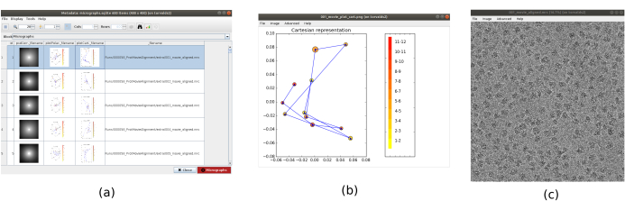
Figure 1. Movie alignment result. (a) The main window of the results, with a list of all the micrographs generated and additional information: the power spectral density, the trajectory of the estimated alignment in polar coordinates, the same in cartesian coordinates, the filename of the generated micrograph. (b) The alignment trajectory represented in cartesian coordinates. (c) The generated micrograph. Please click here to view a larger version of this figure.
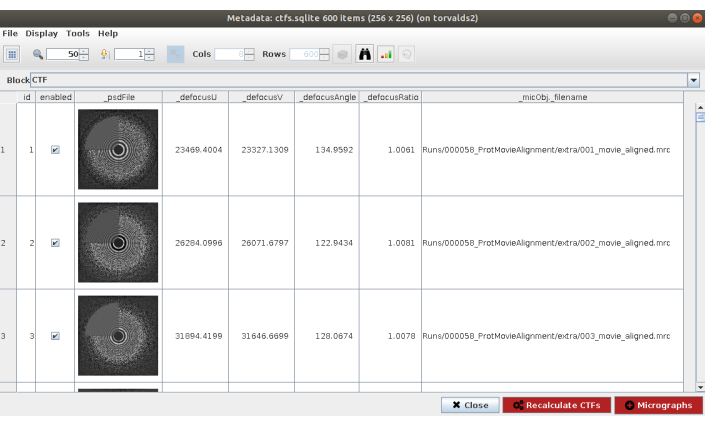
Figure 2. CTF estimation with Ctffind result. The main window with the results includes a figure with the estimated PSD (in a corner) along with the PSD coming from the data, and several defocus params. Please click here to view a larger version of this figure.
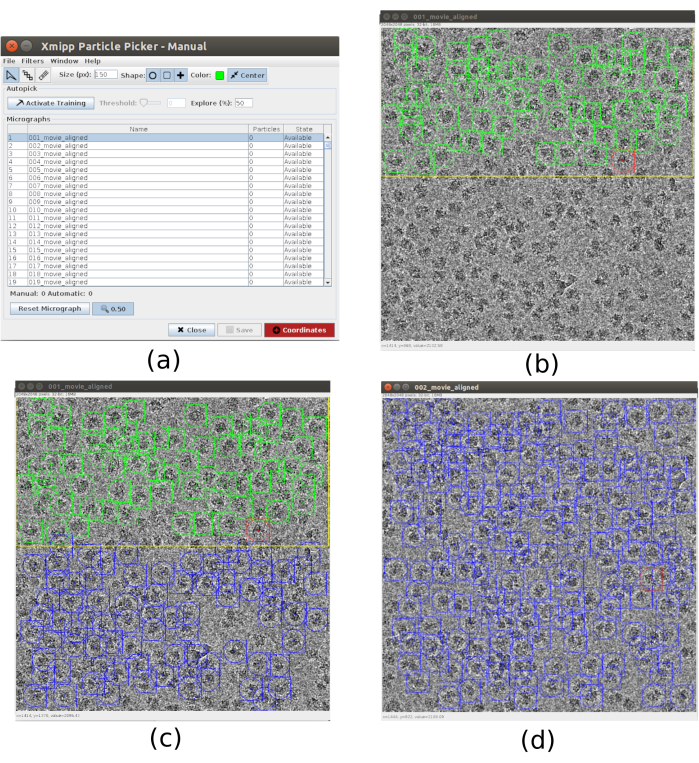
Figure 3. Manual picking windows with Xmipp. (a) The main window with the list of micrographs to process and some other parameters. (b) Manually picking particles inside a region of a micrograph. (c) and (d) Automatically picked particles to be supervised to create a set of training particles for the Xmipp auto picking method. Please click here to view a larger version of this figure.
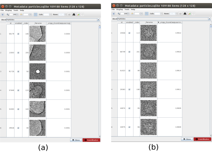
Figure 4. Deep consensus picking with Xmipp result. The parameter zScoreDeepLearning gives weight to the goodness of a particle and it is key to discovering bad particles. (a) The lowest zScores values are associated with artifacts. (b) The highest zScores are associated with particles containing the macromolecule. Please click here to view a larger version of this figure.
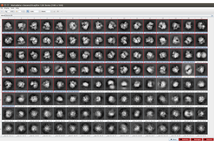
Figure 5. 2D classification with Cryosparc result. The classes generated (averages of subsets of particles coming from the same orientation) are shown. Several good classes selected in red (with some level of detail) and some bad classes non-selected (noisy and uncentered classes). Please click here to view a larger version of this figure.
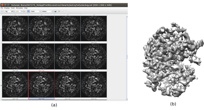
Figure 6. 3D initial volume with swarm consensus result. A view of the 3D initial volume obtained after running the consensus tool xmipp3 - swarm consensus, using the previous 3D initial volume estimations of Xmipp and Relion. (a) The volume is represented by slices. (b) 3D visualization of the volume. Please click here to view a larger version of this figure.
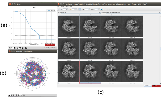
Figure 7. Refinement of a 3D initial volume with Relion result. (a) FSC curve obtained, crossing the threshold at a 4.5Å, approximately. (b) Angular coverage shown as upper view of the 3D sphere. In this case, as there is no symmetry, the assigned particles should cover the whole sphere. (c) Refined volume represented by slices. Please click here to view a larger version of this figure.
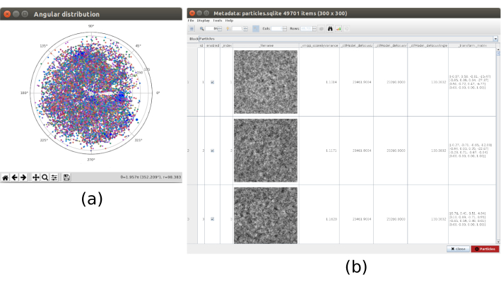
Figure 8. 3D alignment based on deep learning with Xmipp result. The results generated by xmipp3 - deep align method for 3D alignment. (a) The angular assignment for every particle in the form of transformation matrix. (b) The angular coverage. Please click here to view a larger version of this figure.
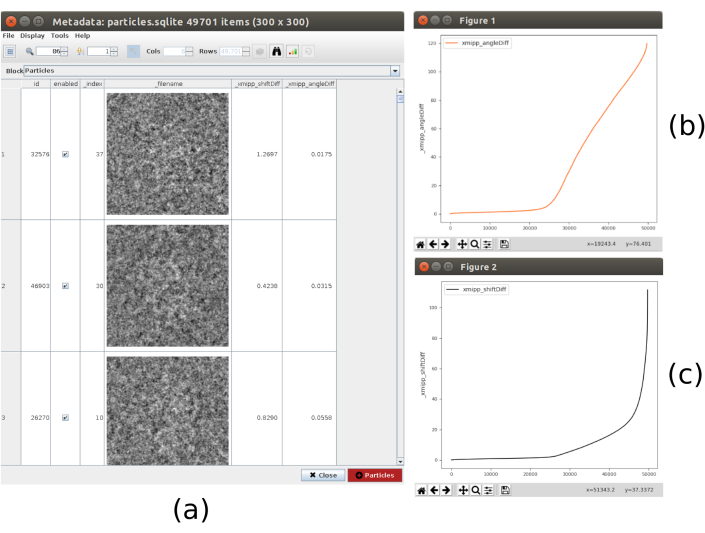
Figure 9. 3D alignment consensus result. (a) List of particles with the obtained differences in shift and angles parameters. (b) Plot of the angular differences per particle. (c) Plot of the shift difference per particle. Please click here to view a larger version of this figure.
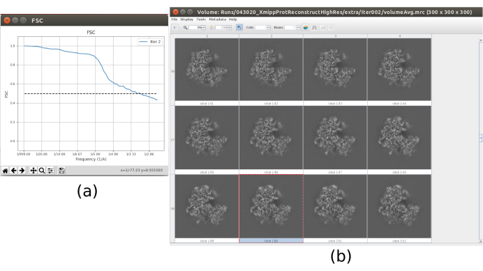
Figure 10. Final iteration of 3D refinement result. (a) FSC curve. (b) Obtained volume at full resolution by slices. Please click here to view a larger version of this figure.
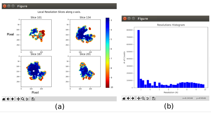
Figure 11. Local resolution analysis with Xmipp result. Results of the method xmipp3 - local MonoRes. (a) Some representative slices colored with the resolution value per voxel, as indicated in the color code. (b) Local resolution histogram. Please click here to view a larger version of this figure.
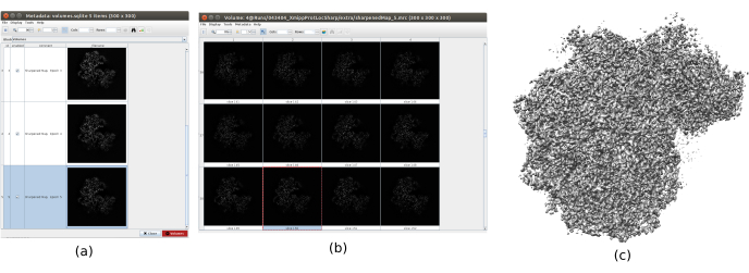
Figure 12. Sharpening with Xmipp result. Results of xmipp3 - localdeblur sharpening method. (a) List of obtained volumes per iteration. (b) 3D volume obtained after the last iteration represented by slices. (c) A 3D representation of the final volume. Please click here to view a larger version of this figure.
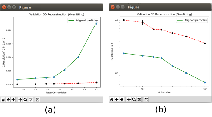
Figure 13. Validate overfitting tool in Xmipp result. Results of xmipp3 - validation overfitting. The green line corresponds to reconstruction from data, the red line from noise. (a) Inverse of the squared resolution with the logarithm of the number of particles. (b) Resolution with the number of particles. Please click here to view a larger version of this figure.

Figure 14. Several 3D representations of the obtained volume. (a) Pre-processed volume. (b) Post-processed volume. (c) Local resolution, dark blue voxels are those with higher resolution (2.75Å) and dark red voxels are those with lower resolution (10.05Å). (d) Zoom in the post-processed volume where an alpha-helix (red oval) can be seen. Please click here to view a larger version of this figure.
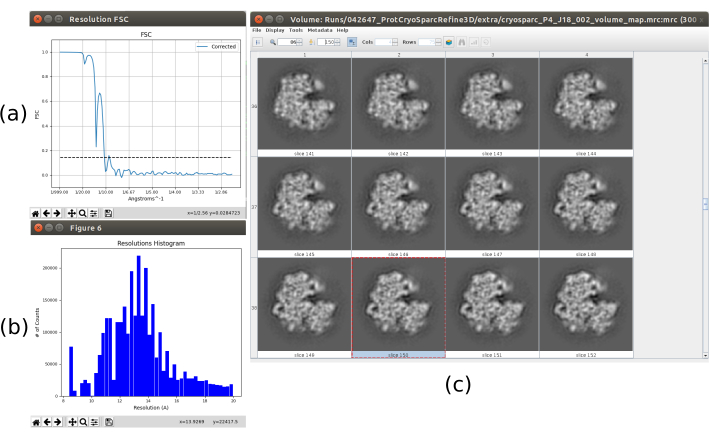
Figure 15. Example of a bad 3D reconstruction. (a) FSC curve with a sharp fall and crossing the threshold at low resolution. (b) Local resolution histogram. (c) 3D volume by slices. Please click here to view a larger version of this figure.

Figure 16. Example of 2D classes. (a) Good classes showing some level of detail. (b) Bad classes containing noise and artifacts (upper part obtained with Xmipp, lower with CryoSparc). Please click here to view a larger version of this figure.
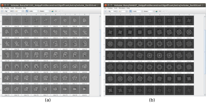
Figure 17. Example of 3D initial volume with different qualities. (a) Good initial volume where the shape of the macromolecule can be observed. (b) Bad initial volume where the obtained shape is completely different from the expected one. Please click here to view a larger version of this figure.
Supplemental Figure 1. Creating a Scipion project. Window displayed by Scipion where an old project can be selected or a new one can be created giving a name and a location for that project. Please click here to download this File.
Supplemental Figure 2. Import movies method. Window displayed by Scipion when pwem - import movies is open. Here, the main acquisition parameters must be included to let the movies available to be processed in Scipion. Please click here to download this File.
Supplemental Figure 3. Movie alignment method. Window displayed by Scipion when xmipp3 - optical alignment is used. The input movies, the range of frames considered for alignment, and some other parameters to process the movies should be filled. Please click here to download this File.
Supplemental Figure 4. CTF estimation method with Ctffind. The form in Scipion with all the necessary fields to run the program Ctffind. Please click here to download this File.
Supplemental Figure 5. Wizard in Scipion. A wizard to help the user filling some parameters in the form. In this case, the wizard is to complete the resolution field in the grigoriefflab - ctffind method. Please click here to download this File.
Supplemental Figure 6. CTF refinement method with Xmipp. The form of xmipp3 - ctf estimation with all the parameters to make a refinement of a previously estimated CTF. Please click here to download this File.
Supplemental Figure 7. Preprocess micrographs method. The form of xmipp3 - preprocess micrographs that allows carrying out some operations over them. In this example, Remove bad pixels and Downsample micrographs is the useful one. Please click here to download this File.
Supplemental Figure 8. Picking method with Cryolo. The form to run the Cryolo picking method using a pretrained network. Please click here to download this File.
Supplemental Figure 9. Consensus picking method with Xmipp. The form of xmipp3 - deep consensus picking based on deep learning to calculate a consensus of coordinates, using a pretrained network over several sets of coordinates obtained with different picking methods. Please click here to download this File.
Supplemental Figure 10. Extract particles method. Input and preprocess tabs of xmipp3 - extract particles. Please click here to download this File.
Supplemental Figure 11. 3D initial volume method with Xmipp. The form of the method xmipp3 - reconstruct significant to obtain an initial 3D map. The Input and Criteria tabs are shown. Please click here to download this File.
Supplemental Figure 12. Resize volume method. The form to make a crop or resize of a volume. In this example, this method is used to generate a full size volume after xmipp3 - reconstruct significant. Please click here to download this File.
Supplemental Figure 13. 3D initial volume with Relion result. A view of the obtained 3D initial volume with relion - 3D initial model method by slices. Please click here to download this File.
Supplemental Figure 14. Refinement of the initial volume with Relion. The form of the method relion - 3D auto-refine. In this example, it was used to refine an initial volume estimated after consensus. The Input and Reference 3D map tabs are shown. Please click here to download this File.
Supplemental Figure 15. 3D classification method. Form of relion - 3D classification. The tabs Input, Reference 3D map, and Optimisation are shown. Please click here to download this File.
Supplemental Figure 16. 3D alignment based on a deep learning method. The form opened for the method xmipp3 - deep align. Here it is necessary to train a network with a training set, then that network will predict the angular assignment per particle. Please click here to download this File.
Supplemental Figure 17. 3D refinement method. Form of the xmipp3 - highres method. Tabs Input and Angular assignment are shown. Please click here to download this File.
Supplemental Figure 18. First iteration of 3D refinement result. (a) FSC curve. (b) Obtained volume (of a smaller size than the full resolution) represented as slices. Please click here to download this File.
Supplemental Figure 19. First iteration of 3D refinement correlation analysis. A new window appears by clicking on the bar icon in the upper part of the window with the list of particles. In Plot columns window a histogram of the desired estimated parameter can be created. Please click here to download this File.
Supplemental Figure 20. Validation overfitting tool. Form of xmipp3 - validate overfitting method. Please click here to download this File.
Discussion
Currently, cryo-EM is a key tool to reveal the 3D structure of biological samples. When good data is collected with the microscope, the available processing tools will allow us to obtain a 3D reconstruction of the macromolecule under study. Cryo-EM data processing is able to achieve near-atomic resolution, which is key to understanding the functional behavior of a macromolecule and is also crucial in drug discovery.
Scipion is a software that allows creating the whole workflow combining the most relevant image processing packages in an integrative way, which helps the traceability and reproducibility of the entire image-processing workflow. Scipion provides a very complete set of tools to carry out the processing; however, obtaining high resolutions reconstructions depends completely on the quality of the acquired data and how these data is processed.
To get a high resolution 3D reconstruction, the first requirement is to obtain good movies from the microscope, which preserve structural information to high resolution. If this is not the case, the workflow will not be able to extract high definition information from the data. Then, a successful processing workflow should be able to extract particles that really correspond to the structure and to find the orientations of these particles in the 3D space. If any of the steps in the workflow fails, the quality of the reconstructed volume will be degraded. Scipion allows for using different packages in any of the processing steps, which helps to find the most adequate approach to process the data. Moreover, thanks to having many packages available, consensus tools, that boost the accuracy by finding an agreement in the estimated outputs of different methods, can be used. Also, it has been discussed in detail in the Representative Results section several validation tools and how to identify accurate and inaccurate results in every step of the workflow, to detect potential problems, and how to try to solve them. There are several checkpoints along the protocol that could help to realize if the protocol is running properly or not. Some of the most relevant are: picking, 2D classification, initial volume estimation, and 3D alignment. Checking the inputs, repeating the step with a different method, or using consensus, are options available in Scipion that the user can use to find solutions when issues appear.
Regarding the previous approaches to package integration in the Cryo-EM field, Appion31 is the only one that allows real integration of different software packages. However, Appion is tightly connected with Leginon32, a system for automated collection of images from electron microscopes. The main difference with Scipion is that data model and storage are less coupled. In such a way, to create a new protocol in Scipion, only a Python script needs to be developed. However, in Appion, the developer must write the script and change the underlying database. In summary, Scipion was developed to simplify maintenance and extensibility.
We have presented in this manuscript a complete workflow for Cryo-EM processing, using the real case dataset of the Plasmodium falciparum 80S Ribosome (EMPIAR entry: 10028, EMDB entry: 2660). The steps covered and discussed here can be summarized as movie alignment, CTF estimation, particle picking, 2D classification, initial map estimation, 3D classification, 3D refinement, evaluation, and post-processing. Different packages have been used and consensus tools were applied in several of these steps. The final 3D reconstructed volume achieved a resolution of 3 Å and, in the post-processed volume, some secondary structures can be distinguished, like alpha-helices, which helps to describe how atoms are arranged in space.
The workflow presented in this manuscript shows how Scipion can be used to combine different Cryo-EM packages in a straightforward and integrative way to simplify the processing, and obtain more reliable result at the same time.
In the future, the development of new methods and packages will keep growing and software like Scipion to easily integrate all of them will be even more important for the researchers. Consensus approaches will be more relevant even then, when plenty of methods with different basis will be available, helping to obtain more accurate estimations of all the parameters involve in the reconstruction process in Cryo-EM. Tracking and reproducibility are key in the research process and easier to achieve with Scipion thanks to having a common framework for the execution of complete workflows.
Disclosures
The authors have nothing to disclose.
Acknowledgements
The authors would like to acknowledge economical support from: The Spanish Ministry of Science and Innovation through Grants: PID2019-104757RB-I00/AEI/10.13039/501100011033, the "Comunidad Autónoma de Madrid" through Grant: S2017/BMD-3817, Instituto de Salud Carlos III, PT17/0009/0010 (ISCIII-SGEFI/ERDF), European Union (EU) and Horizon 2020 through grant: INSTRUCT - ULTRA (INFRADEV-03-2016-2017, Proposal: 731005), EOSC Life (INFRAEOSC-04-2018, Proposal: 824087), iNEXT - Discovery (Proposal: 871037), and HighResCells (ERC - 2018 - SyG, Proposal: 810057). The project that gave rise to these results received the support of a fellowship from "la Caixa" Foundation (ID 100010434). The fellowship code is LCF/BQ/DI18/11660021. This project has received funding from the European Union's Horizon 2020 research and innovation programme under the Marie Skłodowska-Curie grant agreement No. 713673. The authors acknowledge the support and the use of resources of Instruct, a Landmark ESFRI project.
Materials
| Name | Company | Catalog Number | Comments |
| no material is used in this article | - | - | - |
References
- Nogales, E. The development of cryo-EM into a mainstream structural biology technique. Nature Methods. 13 (1), 24-27 (2016).
- Kühlbrandt, W. The Resolution Revolution. Science. 343 (6178), 1443-1444 (2014).
- . 1.15 A structure of human apoferritin obtained from Titan Mono- BCOR microscope Available from: https://www.rcsb.org/structure/7A6A (2021)
- Arnold, S. A., et al. Miniaturizing EM Sample Preparation: Opportunities, Challenges, and "Visual Proteomics". PROTEOMICS. 18 (5-6), 1700176 (2018).
- Faruqi, A. R., McMullan, G. Direct imaging detectors for electron microscopy. Nuclear Instruments and Methods in Physics Research Section A: Accelerators, Spectrometers, Detectors and Associated Equipment. 878, 180-190 (2018).
- Vilas, J. L., et al. Advances in image processing for single-particle analysis by electron cryomicroscopy and challenges ahead. Current Opinion in Structural Biology. 52, 127-145 (2018).
- Martinez, M., et al. Integration of Cryo-EM Model Building Software in Scipion. Journal of Chemical Information and Modeling. 60, 2533-2540 (2020).
- de la Rosa-Trevín, J. M., et al. Scipion: A software framework toward integration, reproducibility and validation in 3D electron microscopy. Journal of Structural Biology. 195, 93-99 (2016).
- de la Rosa-Trevín, J. M., et al. Xmipp 3.0: an improved software suite for image processing in electron microscopy. Journal of Structural Biology. 184, 321-328 (2013).
- Scheres, S. H. W. . Methods in Enzymology. The Resolution Revolution: Recent Advances In cryoEM. , 125-157 (2016).
- Punjani, A., Rubinstein, J. L., Fleet, D. J., Brubaker, M. A. cryoSPARC: algorithms for rapid unsupervised cryo-EM structure determination. Nature Methods. 14, 290-296 (2017).
- Ludtke, S. J. 3-D structures of macromolecules using single-particle analysis in EMAN. Methods in Molecular Biology. 673, 157-173 (2010).
- Shaikh, T. R., et al. SPIDER image processing for single-particle reconstruction of biological macromolecules from electron micrographs. Nature Protocols. 3, 1941-1974 (2008).
- Wagner, T., et al. SPHIRE-crYOLO is a fast and accurate fully automated particle picker for cryo-EM. Communications Biology. 2, (2019).
- Mindell, J. A., Grigorieff, N. Accurate determination of local defocus and specimen tilt in electron microscopy. Journal of Structural Biology. 142, 334-347 (2003).
- Winn, M. D., et al. Overview of the CCP4 suite and current developments. Acta crystallographica. Section D, Biological crystallography. 67, 235-242 (2011).
- Liebschner, D., et al. Macromolecular structure determination using X-rays, neutrons and electrons: recent developments in Phenix. Acta Crystallographica Section D. 75, 861-887 (2019).
- Wong, W., et al. Cryo-EM structure of the Plasmodium falciparum 80S ribosome bound to the anti-protozoan drug emetine. eLife. 3, 03080 (2014).
- Abrishami, V., et al. Alignment of direct detection device micrographs using a robust Optical Flow approach. Journal of Structural Biology. 189, 163-176 (2015).
- Sorzano, C. O. S., Jonic, S., Nunez Ramirez, R., Boisset, N., Carazo, J. M. Fast, robust and accurate determination of transmission electron microscopy contrast transfer function. Journal of Structural Biology. 160, 249-262 (2007).
- Abrishami, V., et al. A pattern matching approach to the automatic selection of particles from low-contrast electron micrographs. Bioinformatics. 29, 2460-2468 (2013).
- Sanchez-Garcia, R., Segura, J., Maluenda, D., Carazo, J. M., Sorzano, C. O. S. Deep Consensus, a deep learning-based approach for particle pruning in cryo-electron microscopy. IUCrJ. 5, 854-865 (2018).
- Sorzano, C. O. S., et al. A clustering approach to multireference alignment of single-particle projections in electron microscopy. Journal of Structural Biology. 171, 197-206 (2010).
- Sorzano, C. O. S., et al. A statistical approach to the initial volume problem in Single Particle Analysis by Electron Microscopy. Journal of Structural Biology. 189, 213-219 (2015).
- Sorzano, C. O. S., et al. Swarm optimization as a consensus technique for Electron Microscopy Initial Volume. Applied Analysis and Optimization. 2, 299-313 (2018).
- Pettersen, E. F., et al. UCSF Chimera--a visualization system for exploratory research and analysis. Journal of computational chemistry. 25, 1605-1612 (2004).
- Sorzano, C. O. S., et al. A new algorithm for high-resolution reconstruction of single particles by electron microscopy. Journal of Structural Biology. 204, 329-337 (2018).
- Vilas, J. L., et al. MonoRes: Automatic and Accurate Estimation of Local Resolution for Electron Microscopy Maps. Structure. 26, 337-344 (2018).
- Ramirez-Aportela, E., et al. Automatic local resolution-based sharpening of cryo-EM maps. Bioinformatics. 36, 765-772 (2020).
- Heymann, J. B. Validation of 3D EM Reconstructions: The Phantom in the Noise. AIMS Biophys. 2, 21-35 (2015).
- Lander, G. C., et al. Appion: An integrated, database-drive pipeline to facilitate EM image processing. Journal of Structural Biology. 166, 95-102 (2009).
- Suloway, C., et al. Automated molecular microscopy: The new Leginon system. Journal of Structural Biology. 151, 41-60 (2005).
Reprints and Permissions
Request permission to reuse the text or figures of this JoVE article
Request PermissionThis article has been published
Video Coming Soon
Copyright © 2025 MyJoVE Corporation. All rights reserved