Measuring the Stiffness of Ex Vivo Mouse Aortas Using Atomic Force Microscopy

Podsumowanie

We present detailed protocols for isolation of aortas from mouse and measurement of their elastic modulus using atomic force microscopy.

Streszczenie

Arterial stiffening is a significant risk factor and biomarker for cardiovascular disease and a hallmark of aging. Atomic force microscopy (AFM) is a versatile analytical tool for characterizing viscoelastic mechanical properties for a variety of materials ranging from hard (plastic, glass, metal, etc.) surfaces to cells on any substrate. It has been widely used to measure the stiffness of cells, but less frequently used to measure the stiffness of aortas. In this paper, we will describe the procedures for using AFM in contact mode to measure the ex vivo elastic modulus of unloaded mouse arteries. We describe our procedure for isolation of mouse aortas, and then provide detailed information for the AFM analysis. This includes step-by-step instructions for alignment of the laser beam, calibration of the spring constant and deflection sensitivity of the AFM probe, and acquisition of force curves. We also provide a detailed protocol for data analysis of the force curves.

Wprowadzenie

The biomechanical properties of arteries are a critical determinant in cardiovascular disease (CVD) and aging. Arterial stiffness, a major cholesterol independent risk factor and an indicator for the progression of CVD, increases with vascular injury, atherosclerosis, age, and diabetes^1-8. Arterial wall stiffening is associated with increased dedifferentiation, migration, and proliferation of vascular smooth muscle cells^9-12. In addition, increased arterial stiffness has been linked to enhanced macrophage adhesion¹, endothelial permeability and leukocyte transmigration¹³, and vessel wall remodeling^14,15. Thus, therapies that could prevent arterial stiffening in CVD or aging might complement currently available pharmacological interventions that treat CVD by reducing high blood cholesterol.

AFM is a powerful analytical tool used for various physical and biological applications. AFM is increasingly used to obtain the high-resolution images and characterize the biomechanical properties of soft biological samples such as tissues and cells^1,2,10,16,17 with a great degree of accuracy at nanoscale levels. A major advantage of AFM is the fact that it can be used with living cells.

This paper describes our method for measuring the elastic modulus of mouse arteries ex vivo using AFM. The described method shows how we 1) properly isolate mouse arteries (descending aorta and aortic arch) and 2) measure the elastic modulus of these tissues by AFM. Measurements of unloaded elastic moduli in arteries can help to elucidate changes in the extracellular matrix (ECM) that occur in response to vascular injury, CVD, and aging.

Protokół

Animal work in this study was approved by the Institutional Animal Care and Use Committees of the University of Pennsylvania. The methods were carried out in accordance with the approved guidelines.

1. Preparing the Mouse and Isolation of the Aorta

1. Anesthetize a mouse with ketamine (80 - 100 mg/kg), xylazine (8 - 10 mg/kg) and acepromazine (1 - 2 mg/kg) intraperitoneally. Confirm anesthesia with a tail pinch test. Once the mouse is fully anesthetized, euthanize the mouse by cervical dislocation.
2. Place the mouse on its back and pin the mouse to a dissection board. Clean the abdomen area with 70% (v/v) ethanol wipes.
3. Pinch the skin at the mid-line and make a small initial incision with medium sized microsurgery scissors at the abdomen. While holding the skin with forceps, use medium sized microsurgery scissors to cut the skin and peritoneum from the abdomen to the sternum.
4. Cut away the ribs on both sides with medium sized microsurgery scissors. Carefully remove the lungs and liver with small sized microsurgery scissors, and leave the heart and aorta. Transfer the mouse and dissection board to a dissecting microscope.
5. Grasp the fat surrounding the aorta with small forceps and use small scissors to carefully cut away fat around the aorta.
6. Gently grab the aorta with forceps, make one cut with small sized microsurgery scissors at the beginning of the ascending aorta and another cut at the end of the descending aorta, just above the abdominal aorta.
7. Transfer the dissected aorta to a 60-mm dish containing 1x phosphate-buffered saline (PBS; without calcium and magnesium).
8. Continue to dissect away any remaining fatty tissue from the aorta using small sized microsurgery scissors. Use small scissors to open the aorta longitudinally.
9. Use small sized microsurgery scissors to cut a small piece (~ 2 x 4 mm) of the descending aorta and aortic arch for AFM analysis (Figure 1). Place the tissue in a 60-mm plastic dish and keep it moist in a drop of PBS .

Figure 1: An Image Showing the Location of the Different Aortic Segments in a Mouse. The aorta was isolated from the heart to the diaphragm, and a small portion of the descending aorta and the aortic arch were used to determine the elastic moduli. Scale bar, 1 mm. Please click here to view a larger version of this figure.

2. Preparing Tissue Samples for the AFM Measurements

1. Carefully remove the PBS using a lab-wipe without touching the aorta. Be certain that the luminal side of the tissue is facing up.
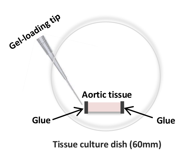
2. Gently glue each end of the opened aorta to the plate by adding 5 - 10 μl of cyanoacrylate adhesive with a gel-loading tip (Figure 2).
   NOTE: The amount of glue needed to firmly attach the tissue at each end must be determined empirically. It is critical that the aorta is not stretched during this process.
3. Check the glued aorta to make certain that it is not folded or floating. After air-drying the glue on the aorta (30 - 60 sec), gently add PBS and submerge the sample.
   NOTE: Preparation the AFM (steps 3 - 5) can be carried out while the tissue is being prepared for analysis.

Figure 2: Cartoon of an Aortic Segment Glued onto a 60-mm Culture Dish using Cyanoacrylate Adhesive. The cyanoacrylate adhesive is being applied to the edge of an aortic sample in preparation for AFM measurements. Please click here to view a larger version of this figure.

3. Loading the Probe

1. Mount a fluid probe holder onto the probe load stand.
2. Using tweezers, slide a silicon nitride AFM probe (0.06 N/m cantilever) with a spherical tip (we have used a 1-µm diameter SiO₂ particle but larger sizes may also be used) on the probe holder. Make sure that the AFM probe is firmly secured to the probe holder.
3. Slide the probe holder onto the Z-scanner mount of the AFM head, and ensure that the probe holder is securely attached.

4. Aligning the Laser on the Probe

1. Open the AFM software. Choose the experiment type on the software; Experiment Category to Contact Mode, Experiment Group to Contact Mode in fluid and Experiment to Contact Mode in fluid. Click Load experiment in the software; this will turn on the laser.
2. Add 3 ml of distilled water to a 50-mm glass bottom dish and place the dish on the stage of the laser alignment unit. This unit simplifies the process of focusing the laser beam onto the back of cantilever.
3. Mount the AFM head in an upright position onto the laser alignment unit and power on the laser alignment unit. Add approximately 50 μl of distilled water to form a droplet on the AFM tip.
4. Using the joystick, lower the AFM head so the AFM tip makes contact with water in the dish. If contact is not made between the AFM tip and water in the dish, gently raise the dish until contact is made. Adjust the focus, brightness and XY position so the AFM tip is in view on the LCD screen of the alignment unit.
5. Position the laser spot onto the tip of the AFM probe by adjusting the laser positioning knobs of the AFM head. Using the detector positioning knobs on the AFM head, adjust the position of the photodiode until values between 0 and -1 V are obtained for the vertical deflection and ~ 0 V is obtained for the horizontal deflection.
6. Check to ensure the laser sum signal is maximized. If necessary, repeat step 4.5 to re-adjust the position of the laser beam on the AFM tip and the position of the photodiode to obtain the maximum sum signal.
   NOTE: It may be necessary to reposition the AFM probe on the probe holder to obtain a maximum sum signal even if step 4.5 is repeated.

5. Calibrating the Deflection Sensitivity and Spring Constant of the AFM Probe

1. Make a scratch on a 60-mm culture dish with a forcep and fill the dish with distilled water. Place the culture dish on the sample holder plate. In this case, mount the dish on the motorized XY scan stage of an inverted microscope.
2. Place a magnetic plate holder on top of the plate to keep it secure during imaging.
3. Click 'Up' arrow in the Navigation menu on the software to move the AFM head up to nearly its highest position to ensure that the AFM probe will not touch the dish.
   NOTE: This step is very important as it avoids breaking the AFM tip.
4. Place the AFM head on the microscope stage.
5. Use the microscope to focus on the scratch on the plate. Use the joystick, or click the 'Down' arrow in the Navigation menu, to slowly and carefully lower the AFM probe into the PBS. Position the head slightly above the scratch in the plate.
   NOTE: If the initial position of the AFM head is closer to the sample, the engage time will be significantly reduced.
6. Before engaging, re-adjust the position of the laser beam on the AFM tip and the position of the photodiode to obtain the maximum SUM signal as necessary.
7. Select a tip type by clicking Change Probe in the Setup menu.
8. Click Check Parameters and set the parameters: Scan Size to 0, Scan Rate to 1 Hz, Sample/line to 256 and Deflection Setpoint to 20 nm. Click Engage. The Engage Status window will remain open until the probe makes contact with the surface of the plate. After engaging the probe, click Ramp.
9. Click Expanded Mode in the Scan Toolbar menu and set the parameters: Ramp Size to between 500 nm and 1 µm, Ramp Rate to 2 Hz, Number of Samples to 256, Tip Radius to 500 nm, Sample Poisson's Ratio to 0.5 (assumes the material to be measured is perfectly incompressible), Tip Half Angle to 0, Trigger Mode to Relative and Trigger Threshold to between 20 and 100 nm.
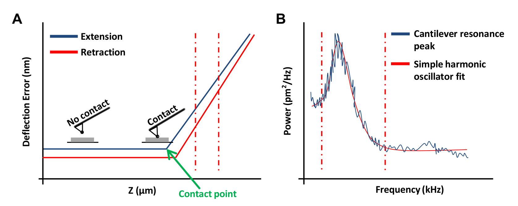
10. Click Ramp Continuous in the Ramp Toolbar menu to obtain a force curve on the plate (Figure 3A). In this force curve, set channel 1 to deflection error.
    NOTE: This will allow the software to graph the results as vertical deflection vs. z position.
    1. Click at the left or right ends of the force curve and drag the cursor to encompass a linear region of the force curve (Figure 3A, dashed red lines). Use these two lines to mark the boundaries of the sloped region to be fit with a straight line.
11. Select Ramp in the Toolbar and click Update Sensitivity. Record the value and repeat this step four more times. Select Calibrate in the Toolbar and then click Detector. Input an average value from the five measurements in the Deflection Sensitivity box.
12. Click Withdraw 2 - 3 times to raise the AFM head. This step is important to prevent interaction between the AFM tip and the plate during the thermal tune process. Click Thermal Tune in the Toolbar.
13. Set Thermal Tune Range of 1 - 100 kHz (This information can be obtained from the manufacturer's catalog) and Deflection Sensitivity Correction to 1.144 for v-shaped cantilevers and 1.106 for rectangular cantilevers.
14. In the Thermal Tune menu, click Acquire Data to obtain a thermal tune curve (Figure 3B). Using the AFM software, place red dashed lines on either side of the curve (as shown in Figure 3B) by dragging the mouse in from the edge of the graph to define the boundaries for fitting. Select either the Lorentzian (Air) or the Simple Harmonic oscillator (Fluid) model depending on which better fits the data.
15. Click Fit Data, then Calculate Spring K and save this value. Repeat the spring constant calibrations several times and use the average value. Click Withdraw several times.
16. Remove the AFM head from the microscope stage and place it on the alignment unit. Remove the dish from the microscope stage.

Figure 3: AFM Force Curves Used in the Calibration of AFM Probes. (A) A representative AFM force curve (a calibration curve). The extension portion of the force curve between the vertical red dashed lines was used to determine the cantilever deflection sensitivity. (B) A simple harmonic oscillator fit graph used to calculate the spring constant of the cantilever as previously described²⁰. Please click here to view a larger version of this figure.

6. Measuring the Elastic Modulus on Mouse Arteries Ex Vivo

1. Place the 60-mm culture dish containing the aortic tissue on the microscope stage, and secure the plate with the magnetic plate holder.
2. Place the AFM head on the microscope stage. Make certain that the AFM probe does not make contact with the aorta but gently makes contact with PBS and forms a meniscus. If necessary, place the AFM head on the alignment unit and click Withdraw until there is enough clearance to prevent contact, then place the AFM head on the microscope stage.
3. Click Navigate. Using the joystick or clicking 'Down' arrow, slowly lower the AFM probe to locate the cantilever above the aorta. Adjust the photodiode position using the detector positioning knobs on the AFM head if necessary.
4. Click Engage to allow the cantilever to make contact with the aorta.
5. Once the aorta is engaged, ensure that the piezo center is stable and click Ramp. If the piezo center is fluctuating, this may be the result of a false engagement. Withdraw the probe and increase the vertical offset of the laser on the photodiode by small increments (~ 0.5 V) and re-engage.
   1. Also, if the probe is far above the sample surface, manually lower the probe closer to the sample surface before re-engaging. If the previous steps do not eliminate the fluctuation, try exchanging the probe.
6. Set the Ramp Size to 3 µm, the Trigger Mode to Relative and the Trigger Threshold to 100 nm and click Ramp Continuous. Observe that the point of contact between the probe and the sample occurs at approximately the center to the lower ¾ of the Z ramp cycle. If this is not observed, disengage from the sample, adjust the Ramp size as needed, and re-engage the sample.
7. Click Microscope in the Menu Bar and then Engage Settings. Change the SPM Withdraw to 30 µm. Click Ramp Continuous in the Ramp Toolbar menu.
8. After observing the force curve, click Capture in the Menu bar and then Capture Filename. Enter a desired file name with the ending ".000" (this will allow additional captured files to increase in number by 1). Select a designated-folder and save the data.
9. Click Capture in the Capture Toolbar menu. Click Withdraw and then Navigate. Use the Joystick or software controls to position the cantilever over another area of the aorta (next to the initially measured point; see Figure 4).
10. Click Engage, Ramp, and Ramp Continuous, respectively. After observing the force curve, click Stop and then Capture.
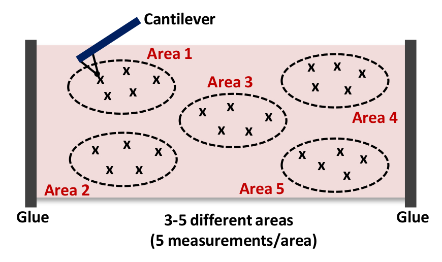
11. Repeat steps 6.9 - 6.10. Capture at least 5 measurements per area as shown in Figure 4. NOTE: We typically collect 15 - 25 force curves from 3 - 5 different locations in each tissue as shown in Figure 4, respectively.

Figure 4: Cartoon of a Cantilever Approaching and Indenting the Tissue (Area 1). This AFM measurement is repeated up to 15 - 25 times from 3 - 5 different locations (Areas 1 - 5) in each artery to acquire the stiffness of the overall tissue sample. Please click here to view a larger version of this figure.

7. Data Analysis

1. Open force curve analysis software.
2. Click Find and Open in the menu bar, and double click on a file to be analyzed.
3. Click Modify Force Parameters in the toolbar menu to check the deflection sensitivity, Spring Constant, Tip Radius, Tip Half Angle and Poisson's ratio. To change the parameters check the box next to it and enter the correct values in the new value column. Then click Execute.
4. If force curves are noisy, click Boxcar Filter and set inputs for Direction to Extend, Average Points to 3 and Filter Order to 0^th. Click Execute to smooth the data.
5. Click Baseline Correction in the menu bar and set inputs for Direction to Extend, Plot Units to Force, Type to Separation, Correction Order to 1^st and Extend Baseline Source to Extend. Adjust the vertical dotted blue lines to encompass the flat portion of force curve and then click Execute.
6. Click Indentation in the toolbar menu and set inputs for Active Curve to Extended, Fit Method to Contact Point Based, Contact Point Algorithm to Treat as Fit Variable, Include Adhesion Force to No, Max Force Fit Boundary to 30%, Min Force Fit Boundary to 0% and Fit Model to Hertzian (Spherical).
   NOTE: In our measurements, significant adhesion between the tip and sample (a negative deflection of the cantilever in the retraction curve) was rarely observed. In cases where such adhesion is observed, the appropriate model (DMT or JKR) should be used for analysis^18,19.
7. Save the values of Young's modulus. Analyze the Young's (elastic) modulus of each of the 3 - 5 areas (5 force curves per area) taken within a small distance of each other as shown in Figure 4.
   NOTE: To remove artifacts, exclude Young's moduli > 100 kPa (normally ~10% of total measurements) from the analysis.
8. Calculate a mean Young's modulus value for each of the 3 - 5 areas (that have been measured) and use these values to calculate a mean elastic modulus for the aorta as a whole.
   NOTE: At least 3 and more often 4 - 6 individual aortas are used to obtain an accurate assessment of arterial stiffness. The final results are plotted as mean + SEM of "n" independent experiments. The exact number of aortas needed will, of course, depend on the level of accuracy required.

Wyniki

Figure 5A shows a phase contrast image of the descending (thoracic) aorta from a 6-month old, male C57BL/6 mouse. The AFM cantilever is in place directly above the tissue and ready for indentation. Figures 5B and 5C demonstrate representative force curves obtained by AFM indentation in contact mode. Green lines shown in Figures 5B and 5C represent the best fit curves obtained using the Hertzian model for a sphere. In Figure 5D

Dyskusje

AFM indentation can be used to characterize the stiffness (elastic modulus) of cells and tissues. In this paper, we provide detailed step-by-step protocols to isolate the descending aorta and aortic arch in the mouse and determine the elastic moduli of these arterial regions ex vivo. We now summarize and discuss the technical issues and limitations of the method described in this paper.

Several technical issues can arise in the isolation and analysis of mouse aortas given their small ...

Materiały

Name	Company	Catalog Number	Comments
BioScope Catalyst AFM system	Bruker
Nikon Eclipse TE 200 inverted microscope	Nikon Instruments
Silicon nitride AFM probe	Novascan Technologies	PT.SI02.SN.1	0.06 N/m cantilever; 1 µm SiO2 particle
Dumont #5 forceps	Fine Science Tools	11251-10	See section 1.4
Dumont #5SF forceps	Fine Science Tools	11252-00	See section 1.8
Fine Scissors-ToughCut	Fine Science Tools	14058-11	See section 1.4 (medium sized)
Vannas-Tübingen spring scissors	Fine Science Tools	15008-08	See section 1.6 (small sized)
60 mm TC-treated cell culture dish	Corning	353004
Dulbecco's Phosphate-Buffered Saline, 1x	Corning	21-031-CM	Without calcium and magnesium
Krazy Glue instant all purpose liquid	Krazy Glue	KG58548R	See section 2.2
Gel-loading tips, 1 - 200 µl	Fisher	02-707-139	See section 2.2
Tip Tweezers	Electron Microscopy Sciences	78092-CP	See section 3.2
50-mm, clear wall glass bottom dishes	TED PELLA	14027-20	See section 4.4