Atomic Force Microscopy Cantilever-Based Nanoindentation: Mechanical Property Measurements at the Nanoscale in Air and Fluid

Summary

Quantifying the contact area and force applied by an atomic force microscope (AFM) probe tip to a sample surface enables nanoscale mechanical property determination. Best practices to implement AFM cantilever-based nanoindentation in air or fluid on soft and hard samples to measure elastic modulus or other nanomechanical properties are discussed.

Abstract

An atomic force microscope (AFM) fundamentally measures the interaction between a nanoscale AFM probe tip and the sample surface. If the force applied by the probe tip and its contact area with the sample can be quantified, it is possible to determine the nanoscale mechanical properties (e.g., elastic or Young's modulus) of the surface being probed. A detailed procedure for performing quantitative AFM cantilever-based nanoindentation experiments is provided here, with representative examples of how the technique can be applied to determine the elastic moduli of a wide variety of sample types, ranging from kPa to GPa. These include live mesenchymal stem cells (MSCs) and nuclei in physiological buffer, resin-embedded dehydrated loblolly pine cross-sections, and Bakken shales of varying composition.

Additionally, AFM cantilever-based nanoindentation is used to probe the rupture strength (i.e., breakthrough force) of phospholipid bilayers. Important practical considerations such as method choice and development, probe selection and calibration, region of interest identification, sample heterogeneity, feature size and aspect ratio, tip wear, surface roughness, and data analysis and measurement statistics are discussed to aid proper implementation of the technique. Finally, co-localization of AFM-derived nanomechanical maps with electron microscopy techniques that provide additional information regarding elemental composition is demonstrated.

Introduction

Understanding the mechanical properties of materials is one of the most fundamental and essential tasks in engineering. For the analysis of bulk material properties, there are numerous methods available to characterize the mechanical properties of material systems, including tensile tests¹, compression tests², and three- or four-point bending (flexural) tests³. While these microscale tests can provide invaluable information regarding bulk material properties, they are generally conducted to failure, and are hence destructive. Additionally, they lack the spatial resolution necessary to accurately investigate the micro- and nanoscale properties of many material systems that are of interest today, such as thin films, biological materials, and nanocomposites. To begin addressing some of the problems with large-scale mechanical testing, mainly its destructive nature, microhardness tests were adopted from mineralogy. Hardness is a measure of the resistance of a material to plastic deformation under specific conditions. In general, microhardness tests use a stiff probe, usually made from hardened steel or diamond, to indent into a material. The resulting indentation depth and/or area can then be used to determine the hardness. Several methods have been developed, including Vickers⁴, Knoop⁵, and Brinell⁶ hardness; each provides a measure of microscale material hardness, but under different conditions and definitions, and as such only produces data that can be compared to tests performed under the same conditions.

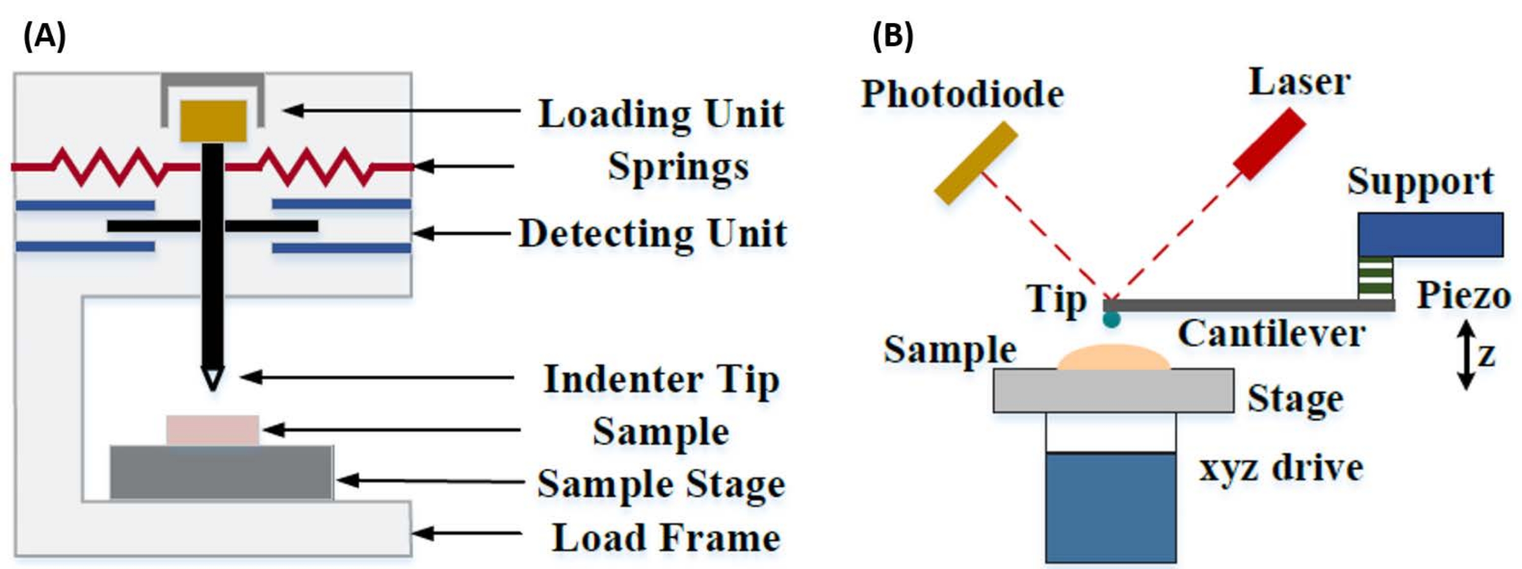
Instrumented nanoindentation was developed to improve upon the relative values obtained via the various microhardness testing methods, improve the spatial resolution possible for the analysis of mechanical properties, and enable the analysis of thin films. Importantly, by utilizing the method first developed by Oliver and Pharr⁷, the elastic or Young's modulus, E, of a sample material can be determined via instrumented nanoindentation. Furthermore, by employing a Berkovich three-sided pyramidal nanoindenter probe (whose ideal tip area function matches that of the Vickers four-sided pyramidal probe)⁸, direct comparison between nanoscale and more traditional microscale hardness measurements can be made. With the growth in popularity of the AFM, AFM cantilever-based nanoindentation began receiving attention as well, particularly for measuring the mechanical properties of softer materials. As a result, as depicted schematically in Figure 1, the two most commonly employed techniques today to interrogate and quantify nanoscale mechanical properties are instrumented nanoindentation (Figure 1A) and AFM cantilever-based nanoindentation (Figure 1B)⁹, the latter of which is the focus of this work.

Figure 1: Comparison of instrumented and AFM cantilever-based nanoindentation systems. Schematic diagrams depicting typical systems for conducting (A) instrumented nanoindentation and (B) AFM cantilever-based nanoindentation. This figure was modified from Qian et al.⁵¹. Abbreviation: AFM = atomic force microscopy. Please click here to view a larger version of this figure.

Both instrumented and AFM cantilever-based nanoindentation employ a stiff probe to deform a sample surface of interest and monitor the resultant force and displacement as a function of time. Typically, either the desired load (i.e., force) or (Z-piezo) displacement profile is specified by the user via the software interface and directly controlled by the instrument, while the other parameter is measured. The mechanical property most often obtained from nanoindentation experiments is the elastic modulus (E), also referred to as the Young's modulus, which has units of pressure. The elastic modulus of a material is a fundamental property relating to the bond stiffness and is defined as the ratio of tensile or compressive stress (σ, the applied force per unit area) to axial strain (ε, the proportional deformation along the indentation axis) during elastic (i.e., reversible or temporary) deformation prior to the onset of plastic deformation (equation [1]):

    (1)

It should be noted that, because many materials (especially biological tissues) are in fact viscoelastic, in reality, the (dynamic or complex) modulus consists of both elastic (storage, in phase) and viscous (loss, out of phase) components. In actual practice, what is measured in a nanoindentation experiment is the reduced modulus, E*, which is related to the true sample modulus of interest, E, as shown in equation (2):

    (2)

Where E_tip and ν_tip are the elastic modulus and Poisson's ratio, respectively, of the nanoindenter tip, and ν is the estimated Poisson's ratio of the sample. The Poisson's ratio is the negative ratio of the transverse to axial strain, and hence indicates the degree of transverse elongation of a sample upon being subjected to axial strain (e.g., during nanoindentation loading), as shown in equation (3):

    (3)

The conversion from reduced to actual modulus is necessary because a) some of the axial strain imparted by the indenter tip may be converted to transverse strain (i.e., the sample may deform via expansion or contraction perpendicular to the direction of loading), and b) the indenter tip is not infinitely hard, and thus the act of indenting the sample results in some (small) amount of deformation of the tip. Note that in the case where E_tip >> E (i.e., the indenter tip is much harder than the sample, which is often true when using a diamond probe), the relationship between the reduced and actual sample modulus simplifies greatly to E ≈ E*(1 - v²). While instrumented nanoindentation is superior in terms of accurate force characterization and dynamic range, AFM cantilever-based nanoindentation is faster, provides orders of magnitude greater force and displacement sensitivity, enables higher resolution imaging and improved indentation locating, and can simultaneously probe nanoscale magnetic and electrical properties⁹. In particular, AFM cantilever-based nanoindentation is superior for the quantification of mechanical properties at the nanoscale of soft materials (e.g., polymers, gels, lipid bilayers, and cells or other biological materials), extremely thin (sub-µm) films (where substrate effects can come into play depending upon indentation depth)^10,11, and suspended two-dimensional (2D) materials^12,13,14 such as graphene^15,16, mica¹⁷, hexagonal boron nitride (h-BN)¹⁸, or transition metal dichalcogenides (TMDCs; e.g., MoS₂)¹⁹. This is due to its exquisite force (sub-nN) and displacement (sub-nm) sensitivity, which is important for accurately determining the initial point of contact and remaining within the elastic deformation region.

In AFM cantilever-based nanoindentation, displacement of an AFM probe toward the sample surface is actuated by a calibrated piezoelectric element (Figure 1B), with the flexible cantilever eventually bending due to the resistive force experienced upon contact with the sample surface. This bending or deflection of the cantilever is typically monitored by reflecting a laser off the back of the cantilever and into a photodetector (position sensitive detector [PSD]). Coupled with the knowledge of the cantilever stiffness (in nN/nm) and deflection sensitivity (in nm/V), it is possible to convert this measured cantilever deflection (in V) into the force (in nN) applied to the sample. Following contact, the difference between the Z-piezo movement and the cantilever deflection yields the sample indentation depth. Combined with the knowledge of the tip area function, this enables calculation of the tip-sample contact area. The slope of the in-contact portions of the resulting force-distance or force-displacement (F-D) curves can then be fit using an appropriate contact mechanics model (see the Data Analysis section of the discussion) to determine the nanomechanical properties of the sample. While AFM cantilever-based nanoindentation possesses some distinct advantages over instrumented nanoindentation as described above, it also presents several practical implementation challenges, such as calibration, tip wear, and data analysis, which will be discussed here. Another potential downside of AFM cantilever-based nanoindentation is the assumption of linear elasticity, as the contact radius and indentation depths need to be much smaller than the indenter radius, which can be difficult to achieve when working with nanoscale AFM probes and/or samples exhibiting significant surface roughness.

Traditionally, nanoindentation has been limited to individual locations or small grid indentation experiments, wherein a desired location (i.e., region of interest [ROI]) is selected and a single controlled indent, multiple indents in a single location separated by some waiting time, and/or a coarse grid of indents are performed at a rate on the order of Hz. However, recent advances in AFM allow for the simultaneous acquisition of mechanical properties and topography through the utilization of high-speed force curve-based imaging modes (referred to by various tradenames depending on the system manufacturer), wherein force curves are conducted at a kHz rate under load control, with the maximum tip-sample force utilized as the imaging setpoint. Point-and-shoot methods have also been developed, allowing for the acquisition of an AFM topography image followed by subsequent selective nanoindentation at points of interest within the image, affording nanoscale spatial control over nanoindentation location. While not the primary focus of this work, specific selected application examples of both force curve-based imaging and point-and-shoot cantilever-based nanoindentation are presented in the representative results, and can be used in conjunction with the protocol outlined below if available on the particular AFM platform employed. Specifically, this work outlines a generalized protocol for the practical implementation of AFM cantilever-based nanoindentation on any capable AFM system and provides four use case examples (two in air, two in fluid) of the technique, including representative results and an in-depth discussion of the nuances, challenges, and important considerations to successfully employ the technique.

Protocol

NOTE: Due to the wide variety of commercially available AFMs and diversity of sample types and applications that exist for cantilever-based nanoindentation, the protocol that follows is intentionally designed to be relatively general in nature, focusing on the shared steps necessary for all cantilever-based nanoindentation experiments regardless of instrument or manufacturer. Because of this, the authors assume the reader possesses at least basic familiarity with operating the specific instrument chosen for performing cantilever-based nanoindentation. However, in addition to the general protocol outlined below, a detailed step-by-step standard operating procedure (SOP) specific to the AFM and software used here (see Table of Materials), focused on cantilever-based nanoindentation of samples in fluid, is included as a Supplementary Material.

1. Sample preparation and instrument setup

1. Prepare the sample in a manner that minimizes both surface roughness (ideally nanometer-scale, ~10x less than the intended indentation depth) and contamination without altering the mechanical properties of the area(s) of interest.
2. Select an appropriate AFM probe for nanoindentation of the intended sample based on the medium (i.e., air or fluid), expected modulus, sample topography, and relevant feature sizes (see the probe selection considerations in the discussion). Load the probe onto the probe holder (see Table of Materials) and attach the probe holder to the AFM scan head.
3. Select an appropriate nanoindentation mode in the AFM software that affords user control of individual ramps (i.e., force-displacement curves).
   NOTE: The specific mode will differ across different AFM manufacturers and individual instruments (see SOP provided in the Supplementary Material for more details and a specific example).
4. Align the laser onto the back of the probe cantilever, opposite the location of the probe tip and into the PSD.
   NOTE: See the mesenchymal stem cell application example for more details regarding important considerations when aligning the laser and conducting nanoindentation in fluid, in particular, avoiding floating debris and/or air bubbles, which can scatter or refract the beam. The AFM optics may also need to be adjusted to compensate for the index of refraction of the fluid and to avoid crashing the probe when engaging the surface.
   1. Center the laser beam spot on the back of the cantilever by maximizing the sum voltage (Figure 2A).
   2. Center the reflected laser beam spot on the PSD by adjusting the X and Y (i.e., horizontal and vertical) deflection signals to be as close to zero as possible (Figure 2A), thereby providing the maximum detectable deflection range for producing an output voltage proportional to the cantilever deflection.
5. If unsure of the sample topography, surface roughness, and/or surface density (in the case of flakes or particles), perform an AFM topography survey scan prior to any nanoindentation experiments to confirm sample suitability, as described in step 1.1 and the sample preparation portion of the discussion.

Figure 2: Position-sensitive detector monitor. (A) PSD display indicating a properly aligned laser reflecting off the back of the probe cantilever and onto the center of the PSD (as evidenced by the large sum voltage and lack of vertical or horizontal deflection) prior to engaging on the sample surface (i.e., probe out of contact with the sample). (B) The vertical deflection voltage increases when the cantilever is deflected (e.g., when the probe makes contact with the sample). Abbreviations: PSD = position-sensitive detector; VERT = vertical; HORIZ = horizontal; AMPL = amplitude; n/a = not applicable. Please click here to view a larger version of this figure.

2. Probe calibration

NOTE: Three values are necessary to quantify the mechanical properties of a sample using the F-D curve data collected during cantilever-based nanoindentation: the deflection sensitivity (DS) of the cantilever/PSD system (nm/V or V/nm), the cantilever spring constant (nN/nm), and the probe contact area, often expressed in terms of the effective probe tip radius (nm) at a given indentation depth less than the probe radius in the case of a spherical probe tip.

1. Calibrate the DS of the probe/AFM system by ramping on an extremely hard material (e.g., sapphire, E = 345 GPa) so that deformation of the sample is minimized and thus the measured Z movement of the piezo following the initiation of tip-sample contact is converted solely into cantilever deflection.
   NOTE: The DS calibration must be performed under the same conditions as the planned nanoindentation experiments (i.e., temperature, medium, etc.) to accurately reflect the DS of the system during the experiments. A long (30 min) laser warmup period may be necessary for maximum accuracy to allow time for thermal equilibrium to be reached and stable laser output power and pointing stability to be established. The DS must be remeasured every time the laser is realigned, even if the same probe is used, as the DS depends on the laser intensity and position on the cantilever, as well as the quality of the reflection from the probe (i.e., degradation of the probe's backside coating will affect the DS) and sensitivity of the PSD²⁰.
   1. Set up and perform the DS calibration indents on the sapphire to achieve approximately the same probe deflection (in V or nm) as the planned sample indents, since the measured displacement is a function of the tip deflection angle and becomes nonlinear for large deflections.
   2. Determine the DS (in nm/V), or alternatively, the inverse optical lever sensitivity (in V/nm), from the slope of the linear portion of the in-contact regime after the initial contact point in the resulting F-D curve, as shown in Figure 3A.
   3. Repeat the ramp at least 5x, recording each DS value. Use the average of the values for maximum accuracy. If the relative standard deviation (RSD) of the measurements exceeds ~1%, remeasure the DS, as sometimes the first few F-D curves are nonideal due to the initial introduction of adhesive forces.
   4. If the probe cantilever's spring constant, k, is not factory-calibrated (e.g., via laser Doppler vibrometry [LDV]), calibrate the spring constant.
      NOTE: The thermal tune method is optimal for relatively soft cantilevers with k < 10 N/m (see the spring constant section of the discussion for a list and description of alternative methods, particularly for stiff cantilevers with k > 10 N/m). As shown in Figure 3B, C, thermal tuning is typically integrated into the AFM control software.
2. If the probe does not come with a factory-calibrated tip radius measurement (e.g., via scanning electron microscope [SEM] imaging), measure the effective tip radius, R.
   NOTE: There are two common methods for measuring the tip radius (see corresponding discussion section), but the most common for nanometer-scale probe tips is the blind tip reconstruction (BTR) method, which utilizes a roughness standard (see Table of Materials) containing numerous extremely sharp (sub-nm) features that serve to effectively image the tip, rather than the tip imaging the sample.
   1. If employing the BTR method, image the roughness (tip characterization) sample using a slow scan rate (<0.5 Hz) and high feedback gains to help optimize tracking of the very sharp features. Choose an image size and pixel density (resolution) based on the expected tip radius (e.g., a 1024 x 1024 pixel image of a 3 µm x 3 µm area will have ~3 nm lateral resolution).
   2. Use AFM image analysis software (see Table of Materials) to model the probe tip and estimate its end radius and effective tip diameter at the expected sample indentation depth, as shown in Figure 3D-F.
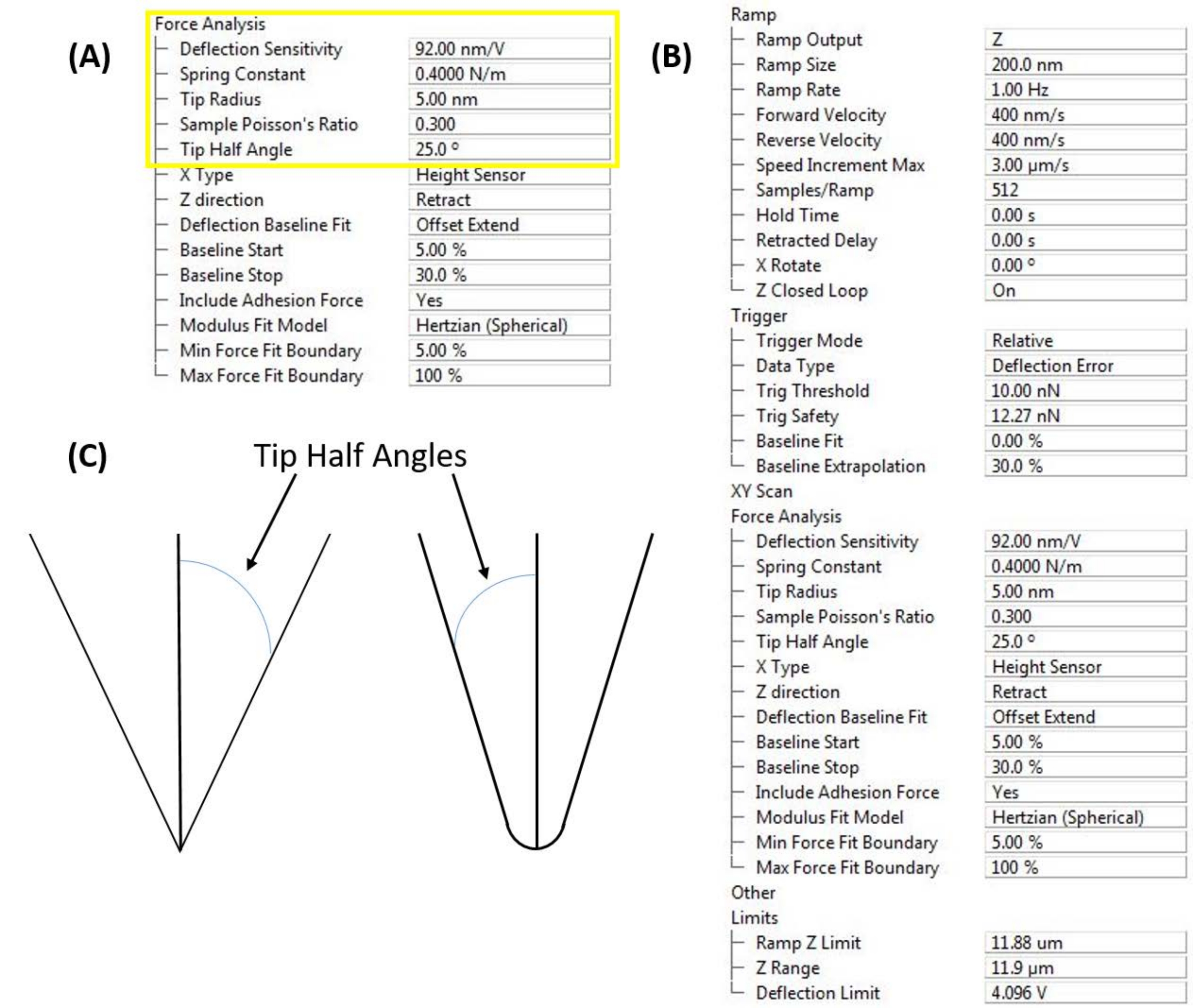
3. Upon completing the probe calibration, enter the DS, k, and R values in the instrument software, as shown in Figure 4A.
   1. Enter an estimate of the sample's Poisson's ratio, ν, to enable converting the measured reduced modulus to the actual sample modulus⁹. If employing a conical or conispherical contact mechanics model based on the tip shape and indentation depth, it is also necessary to enter the tip half angle (Figure 4C).
      NOTE: The modulus is relatively insensitive to small errors or uncertainties in the estimated Poisson's ratio. An estimate of ν = 0.2-0.3 is a good starting point for many materials²¹.

Figure 3: Probe calibration. (A) Deflection sensitivity determination. Result of a representative deflection sensitivity measurement carried out on a sapphire substrate (E = 345 GPa) for a standard tapping mode probe (nominal k = 42 N/m; see Table of Materials) with a reflective backside aluminum coating. Shown are the measured approach (blue trace) and retract or withdraw (red trace) curves. The measured deflection sensitivity of 59.16 nm/V was determined by fitting the approach curve between the snap-to-contact and turn-around points, as indicated by the region between the vertical dotted red lines. The region of negative-going deflection evident in the retract/withdraw curve prior to pulling off the surface is indicative of tip-sample adhesion. (B,C) Thermal tuning. Representative cantilever thermal noise spectra (blue traces) with corresponding fits (red traces) for two different probes. (B) Thermal tune setup and fit parameters for a standard force curve-based AFM imaging probe (see Table of Materials) with its nominal spring constant k = 0.4 N/m used as an initial guess. The fit of the cantilever thermal noise spectrum yields a fundamental resonance frequency of f₀ = 79.8 kHz, which is in reasonably good agreement with the nominal value of f₀ = 70 kHz. The measured Q factor is 58.1. Goodness of fit (R² = 0.99) is based on agreement of the fit with the data between the two vertical dashed red lines. Note that it is important to know and enter both the ambient temperature and deflection sensitivity for accurate results. (C) Cantilever thermal noise spectrum and corresponding fit (i.e., thermal tune) with resultant calculated spring constant k = 0.105 N/m for an extremely soft cantilever used for performing nanomechanical measurements on live cells and isolated nuclei. Note the significantly lower natural resonance frequency of ~2-3 kHz. (D-F) Blind tip reconstruction. Representative blind tip reconstruction workflow for a diamond tip probe (nominal R = 40 nm; see Table of Materials). (D) A 5 µm x 5 µm image of a tip characterization sample consisting of a series of extremely sharp (sub-nm) titanium spikes that serve to image the AFM probe tip. (E) Resultant reconstructed model (inverted height image) of the probe tip. (F) Blind tip reconstruction fitting results, including an estimated end radius of R = 29 nm and effective tip diameter of 40 nm at a user selected height of 8 nm (i.e., indentation depth << R) from the tip apex, calculated by converting the tip-sample contact area at that height into an effective diameter assuming a circular profile (i.e., A = πr² = π(d/2)²) for use with spherical contact mechanics models. Abbreviations: AFM = atomic force microscopy; ETD = effective tip diameter. Please click here to view a larger version of this figure.

Figure 4: Software interface inputs. (A) Probe calibration constants. Software user interface (see Table of Materials) to enter measured deflection sensitivity, spring constant, and tip radius to enable quantitative nanomechanical measurements. The Poisson's ratio of both the probe and sample are necessary for calculating the elastic or Young's modulus of the sample from the cantilever-based nanoindentation force curves. (B) Ramp control window. Software user interface (see Table of Materials) for setting up cantilever-based nanoindentation experiments, organized into the parameters describing the ramp itself (i.e., indentation profile), instrument triggering (e.g., force vs. displacement control), subsequent force analysis, and movement limits (to improve measurement sensitivity by narrowing the range over which the A/D converter has to operate in controlling the Z-piezo and reading the PSD deflection). (C) The tip half angle (based on the probe geometry or direct measurement) is important if a conical, pyramidal, or conispherical contact mechanics model (e.g., Sneddon) is employed. Please click here to view a larger version of this figure.

3. Collect force-displacement (F-D) data

NOTE: The parameter values presented here (see Figure 4B) may vary depending upon the force and indentation range for a given sample.

1. Navigate the sample under the AFM head and engage on the desired region of interest.
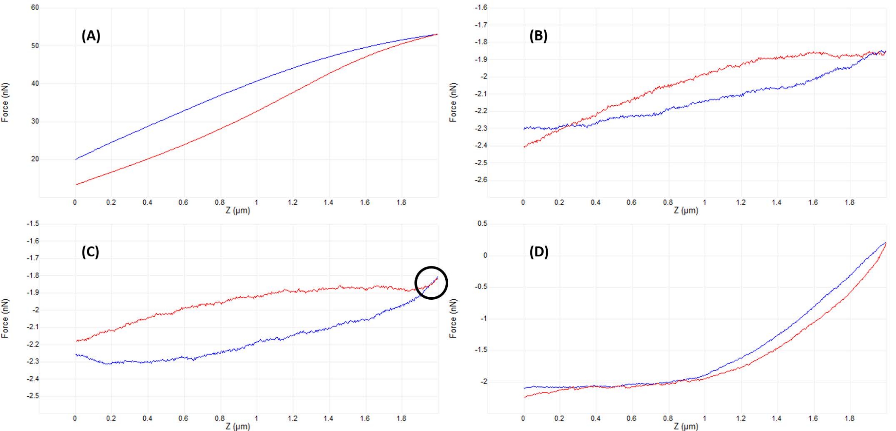
   1. Monitor the vertical deflection signal (Figure 2B) or perform a small (~50-200 nm) initial ramp (Figure 4B) to verify that the tip and sample are in contact (see Figure 5A).
   2. Adjust the AFM head position slightly upward (in steps corresponding to ~50% of the full ramp size) and ramp again. Repeat until the tip and sample are just out of contact, as evidenced by a nearly flat ramp (Figure 5B) and minimal vertical deflection of the cantilever (Figure 2A).
   3. Once no obvious tip-sample interaction is present (compare Figure 2A and Figure 2B), lower the AFM head by an amount corresponding to ~50%-100% of the ramp size to ensure the probe tip will not crash into the sample while manually moving the AFM head. Ramp again, repeating until either a good curve (Figure 5D) or a curve similar to Figure 5C is observed. In the latter case, perform one additional small AFM head-lowering adjustment equal to ~20%-50% of the ramp size to achieve good contact and a force curve similar to that shown in Figure 5D.
2. Adjust ramp parameters (as described below and shown in Figure 4B) to optimize for the instrument, probe, and sample, and obtain ramps similar to that shown in Figure 5D.
   1. Select an appropriate ramp size (i.e., total Z-piezo movement through one ramp cycle) depending on the sample (e.g., thickness, expected modulus, surface roughness) and desired indentation depth.
      NOTE: For stiffer samples, less sample deformation (and hence more probe deflection for a given Z-piezo movement) is likely to occur, so the ramp size can generally be smaller than for softer samples. Typical ramp sizes for stiff samples and cantilevers may be tens of nm, while for soft samples and cantilevers ramps may be hundreds of nm to a few µm in size; specific selected application examples are presented in the representative results section. Note that minimum and maximum possible ramp sizes are instrument-dependent.
   2. Select an appropriate ramp rate (1 Hz is a good starting point for most samples).
      NOTE: The ramp rate may be limited by control and/or detection electronic speeds/bandwidths. In combination with the ramp size, the ramp rate determines the tip velocity. The tip velocity is particularly important to consider when indenting soft materials where viscoelastic effects may cause hysteresis artifacts^9,22.
   3. Choose whether to employ a triggered (load-controlled) or untriggered (displacement-controlled) ramp.
      NOTE: In a triggered ramp, the system will approach the sample in user-defined steps (based on the ramp size and resolution or number of data points) until the desired trigger threshold (i.e., setpoint force or cantilever deflection) is detected, at which point the system will retract to its original position and display the F-D curve. In an untriggered ramp, the system simply extends the Z-piezo the distance specified by the user defined ramp size and displays the measured F-D curve. Triggered ramps are preferred for most use cases, but untriggered ramps can be useful when investigating soft materials that do not exhibit a sharp, easily identifiable contact point.
      1. If a triggered ramp is chosen, set the trigger threshold (user-defined maximum allowed force or deflection of the ramp) to result in the desired indentation into the sample.
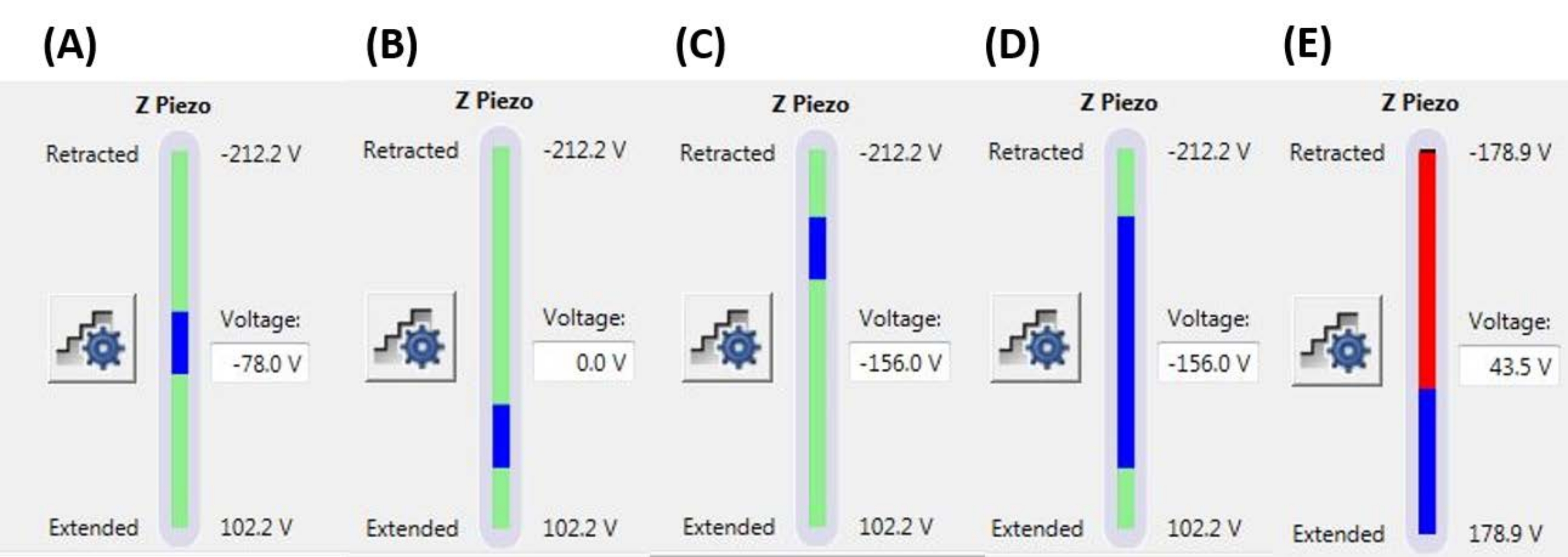
         NOTE: Use of a trigger threshold means that a ramp may terminate (i.e., the probe may begin to retract) before reaching the full ramp size (Z-piezo extension) specified. Values may range from a few nN to a few µN, depending on the tip-sample system.
      2. Set the ramp position to determine the portion of the Z-piezo's maximum range that will be used to execute the ramp. Ensure that the total range of the ramp size does not start or end outside of the maximum Z-piezo range (see representative examples in Figure 6), otherwise a portion of the F-D curve will not represent any physical measurement (i.e., the Z-piezo will be fully extended or retracted, not moving).
   4. Set the number of samples/ramp (e.g., 512 samples/ramp) to achieve the desired resolution of the measurement (i.e., point density of the F-D curve).
      NOTE: The maximum samples/ramp may be limited by software (file size) or hardware constraints (e.g., analog to digital [A/D] conversion speed, depending upon the ramp rate). It is also possible to limit the allowable Z-piezo or deflection range (see limits parameters in Figure 4B) to increase the effective resolution of the system's A/D converter.
   5. Set the X-rotate to reduce the shear forces on the sample and tip by simultaneously moving the probe slightly in the X-direction (parallel to the cantilever) while indenting in the Z-direction (perpendicular to cantilever). Use a value for the X-rotate equal to the offset angle of the probe holder relative to the surface normal (12° is typical).
      NOTE: The X-rotate is necessary because the cantilever is mounted in the probe holder at a small angle relative to the surface to allow the incident laser beam to reflect into the PSD. Additionally, the front and back angles of the probe tip may differ from each other (i.e., the probe tip may be asymmetrical). More specific information can be obtained from individual probe and AFM manufacturers.

Figure 5: Optimizing tip-sample separation after engaging to obtain good force curves. Sequential examples of representative force-displacement curves obtained while indenting in fluid (phosphate-buffered saline) on a live mesenchymal stem cell nucleus with a calibrated soft silicon nitride cantilever (nominal k = 0.04 N/m) terminating in a 5 µm radius hemispherical tip (see Table of Materials). Curves were obtained in the process of engaging the cell surface and optimizing the indentation parameters, with probe approach shown in blue and retract/withdraw in red. (A) The tip is already engaged and in contact with the sample prior to beginning the ramp, leading to large cantilever deflection and forces, with no flat precontact baseline. (B) After manually moving the tip sufficiently far away from the sample, an untriggered 2 µm ramp results in an F-D curve that is nearly flat (i.e., virtually no change in force). In ambient conditions, the curve would be flatter, but in fluid, the viscosity of the medium can cause slight deflections of the probe cantilever during a ramp as seen here, even with no surface contact. (C) After approaching slightly closer to the surface prior to beginning the ramp, the approach and retract curves show a slight increase in force (increased slope) near the turnaround point of the ramp (i.e., transition from approach to withdraw). The telltale sign to look for is that the approach (blue) and withdraw (red) curves begin to overlap (region indicated by the black circle), which is indicative of a physical interaction with the surface. (D) An ideal F-D curve acquired after optimization of the ramp parameters and approaching slightly (~1 µm) closer to the cell surface than in C so that the probe spends approximately half the ramp in contact with the cell, enabling sufficient deformation to fit the contact portion of the approach curve and determine the elastic modulus. The relatively long, flat, low-noise baseline makes it easier for the fitting algorithm to determining the contact point. Abbreviation: F-D = force-displacement. Please click here to view a larger version of this figure.

Figure 6: Ramp size and position. Z-piezo monitor showing the extent of the ramp (blue bar) relative to the total available Z-piezo movement range (green bar). (A) The Z-piezo position is near the middle of its range of movement, as indicated both by the blue bar being located roughly in the middle of the green bar and the current Z-piezo voltage (-78.0 V) being roughly between its fully retracted (-212.2 V) and extended (+102.2 V) values. (B) Z-piezo is extended relative to A, with no bias voltage applied. (C) Z-piezo is retracted relative to A and B. (D) The Z-piezo position is the same as in C at -156.0 V, but the ramp size has been increased relative to A-C to take advantage of more of the Z-piezo's full range of motion. € The ramp size is too large for the current ramp position, resulting in the Z-piezo being extended to the end of its range. This will cause the F-D curve to flatline as the system cannot extend the Z-piezo further. Abbreviation: F-D = force-displacement. Please click here to view a larger version of this figure.

4. F-D curve analysis

1. Choose an appropriate data analysis software package. Select and load the data to be analyzed.
   NOTE: Many AFM manufacturers and AFM image processing software programs have built-in support for F-D curve analysis. Alternatively, the increased flexibility and features of a dedicated F-D curve analysis package, such as the open source AtomicJ software package, may be beneficial²³, particularly for batch processing and statistical analysis of large datasets or implementing complex contact mechanics models.
2. Input calibrated values for the spring constant, DS, and probe tip radius, along with estimates of the Young's modulus and Poisson's ratio for the probe tip (based on its material composition) and the Poisson's ratio of the sample.
   NOTE: If using a diamond tip indenter, the values E_tip = 1140 GPa and ν_tip = 0.07 can be used^21,24,25,26. For a standard silicon probe, E_tip = 170 GPa and ν_tip = 0.27 can typically be used, although the Young's modulus of silicon varies depending upon the crystallographic orientation²⁷.
3. Choose a nanoindentation contact mechanics model appropriate for the tip and sample.
   NOTE: For the many common spherical tip models (e.g., Hertz, Maugis, DMT, JKR), it is imperative that the indentation depth into the sample is less than the tip radius; otherwise the spherical geometry of the probe tip gives way to a conical or pyramidal shape (Figure 4C). For conical (e.g., Sneddon²⁸) and pyramidal models, the tip half angle (i.e., the angle between the side wall of the tip and a bisecting line perpendicular to the tip end; Figure 4C) must be known and is usually available from the probe manufacturer. For more information regarding contact mechanics models, please see the Data Analysis section of thedDiscussion.
4. Run the fitting algorithm. Check for proper fitting of the F-D curves; a low residual error corresponding to an average R² near unity (e.g., R² > 0.9) is typically indicative of a good fit to the chosen model^29,30. Spot check individual curves to visually inspect the curve, model fit, and calculated contact points if desired (e.g., see Figure 7 and the Data Analysis section of the discussion).

Results

Force-displacement curves
Figure 7 shows representative, near-ideal F-D curves obtained from nanoindentation experiments performed in air on resin-embedded loblolly pine samples (Figure 7A) and in fluid (phosphate-buffered saline [PBS]) on mesenchymal stem cell (MSC) nuclei (Figure 7B). The use of any contact mechanics model relies on the accurate and reliable determination of the initial tip-sample contact po...

Discussion

Sample preparation
For nanoindentation in air, common preparation methods include cryosectioning (e.g., tissue samples), grinding and/or polishing followed by ultramicrotoming (e.g., resin-embedded biological samples), ion milling or focused ion beam preparation (e.g., semiconductor, porous, or mixed hardness samples not amenable to polishing), mechanical or electrochemical polishing (e.g., metal alloys), or thin film deposition (e.g., atomic layer or chemical vapor deposition, molecular beam epita...

Materials

Name	Company	Catalog Number	Comments
Atomic force microscope	Bruker	Dimension Icon	Uses Nanoscope control software, including PeakForce Quantitative Nanomechanical Mapping (PF-QNM), FastForce Volume (FFV), and Point-and-Shoot Ramping experimental workspaces
AtomicJ	American Institute of Physics	https://doi.org/10.1063/1.4881683	Flexible, powerful, free open source Java-based force curve analysis software package. Supports numerous contact mechanic models, such as Hertz, Sneddon DMT, JKR, Maugis, and cone or pyramid (including blunt and truncated). Also includes a variety of initial contact point estimation methods to choose from. Supports batch processing of data and subsequent statistical analysis (e.g., averages, standard deviations, histograms, goodness of fit, etc.). Literature citation is: P. Hermanowicz, M. Sarna, K. Burda, and H. Gabry, “AtomicJ: An open source software for analysis of force curves” Rev. Sci. Instrum. 85: 063703 (2014), https://doi.org/10.1063/1.4881683
Buffer solution (PBS)	Fisher Chemical (NaCl), Sigma Aldrich (KCl), Fisher BioReagents (Na2HPO4 and KH2PO4)	S271 (>99% purity NaCl), P9541 (>99% purity KCl), BP332(>99% purity Na2HPO4), BP362 (>99% purity KH2PO4)	Phosphate buffered saline (PBS) was prepared in the laboratory as an aqueous solution consisting of 137 mM NaCl, 2.7 mM KCl, 10 mM Na2HPO4, and 1.8 mM KH2PO4 dissolved in ultrapure water. Reagents were measured out using an analytical balance, and glassware was cleaned with soap and water followed by autoclaving immediately prior to use.
Chloroform
Diamond tip AFM probe	Bruker	PDNISP	Pre-mounted factory-calibrated cube corner diamond (E = 1140 GPa) tip AFM probe (nominal R = 40 nm) with a stainless steel cantilever (nominal k = 225 N/m, f0 = 50 kHz). Spring constant is measured at the factory (k = 256 N/m for the probe, Serial #13435414, used here) and calibration data (including AFM images of indents showing probe geometry) is provided with the probe.
Diamond ultramicrotome blade	Diatome	Ultra 35°	2.1 mm width. Also used a standard glass blade for intial rough cut of sample surface before transitioning to diamond blade for final surface preparation
Epoxy	Gorilla Glue	26853-31-6	Epoxy resin and hardner were mixed in a 1:1 ratio, a small drop was placed on a stainless steel sample puck (Ted Pella), and V1 grade muscovite mica (Ted Pella) was attached to create an atomically flat surface for preparation of phospholipid membranes.
Ethanol
LR white resin, medium grade (catalyzed)	Electron Microscopy Sciences	14381	500 mL bottle, Lot #150629
Mesenchymal stem cells (MSCs)	N/A	N/A	MSCs for nanomechanical studies were primary cells harvested from 8-10 week old male C57BL/6 mice as described in Goelzer, M. et al. "Lamin A/C Is Dispensable to Mechanical Repression of Adipogenesis" Int J Mol Sci 22: 6580 (2021) doi:10.3390/ijms22126580 and Peister, A. et al. "Adult stem cells from bone marrow (MSCs) isolated from different strains of inbred mice vary in surface epitopes, rates of proliferation, and differentiation potential" Blood 103: 1662-1668 (2004), doi:10.1182/blood-2003-09-3070.
Modulus standards	Bruker	PFQNM-SMPKIT-12M	Used HOPG (E = 18 GPa) and PS (E = 2.7 GPa). Also contains 2x PDMS (Tack 0, E = 2.5 MPa; Tack 4, E = 3.5 MPa), PS-LDPE (E = 2.0/0.2 GPa), fused silica (E = 72.9 GPa), sapphire (E - 345 GPa), and tip characterization (titanium roughness) sample. All samples come pre-mounted on a 12 mm diameter steel disc (sample puck).
Muscovite mica	Ted Pella	50-12	12 mm diameter, V1 grade muscovite mica
Nanscope Analysis	Bruker	Version 2.0	Free AFM image processing and analysis software package, but designed for, and proprietary/limited to Bruker AFMs; similar functionality is available from free, platform-independent AFM image processing and analysis software packages such as Gwyddion, WSxM, and others. Has built-in capabilities for force curve analysis, but AtomicJ is more flexible/full featured (e.g., more built-in contact mechanics models to choose from, statistical analysis of force curve fitting results, etc.) for force curve analysis and handles batch processing of force curves.
Phospholipids: POPC, Cholesterol (ovine)	Avanti Polar Lipids	POPC: CAS # 26853-31-6, Cholesterol: CAS # 57-88-5	POPC lipid dissolved in chloroform (25 mg/mL) was obtained from vendor and used without further purification. Cholesterol powder from the same vendor was dissolved in chloroform (20 mg/mL).
Probe holder (fluid, lipid bilayers)	Bruker	MTFML-V2	Specific to the particular AFM used; MTFML-V2 is a glass probe holder for scanning in fluid on a MultiMode AFM.
Probe holder (fluid, MSCs)	Bruker	FastScan Bio Z-scanner	Used with Dimension FastScan head (XY flexure scanners). Serial number MXYPOM5-1B154.
Probe holder (standard, ambient)	Bruker	DAFMCH	Specific to the particular AFM used; DAFMCH is the standard contact and tapping mode probe holder for the Dimension Icon AFM, suitable for nanoindentation (PF-QNM, FFV, and point-and-shoot ramping)
Sample Puck	Ted Pella	16218	Product number is for 15 mm diameter stainless steel sample puck. Also available in 6 mm, 10 mm, 12 mm, and 20 mm diameters at https://www.tedpella.com/AFM_html/AFM.aspx#anchor842459
Sapphire substrate	Bruker	PFQNM-SMPKIT-12M	Extremely hard surface (E = 345 GPa) for measuring deflection sensitivity of probes (want all of the deflection to come from the probe, not the substrate). Part of the PF-QNM/modulus standards kit.
Scanning electron microscope	Hitachi	S-3400N-II	Located at Boise State. Used to perform co-localized SEM/EDS on all samples except additively manufactured (AM) Ti-6Al-4V.
Silicon AFM probes (standard)	NuNano	Scout 350	Standard tapping mode silicon probe with reflective aluminum backside coating; k = 42 N/m (nominal), f0 = 350 kHz. Nominal R = 5 nm. Also available uncoated or with reflective gold backside coating. Probes with similar specifications are available from other manufacturers (e.g., Bruker TESPA-V2).
Silicon AFM probes (stiff)	Bruker	RTESPA-525, RTESPA-525-30	Rotated tip etched silicon probes with reflective aluminum backside coating; k = 200 N/m (nominal), f0 = 525 kHz. Nominal R = 8 nm for RTESPA-525, R = 30 nm for RTESPA-525-30. Spring constant of each RTESPA-525-30 is measured individually at the factory via laser Doppler vibrometry and supplied with the probe.
Silicon carbide grit paper (abrasive discs)	Allied	50-10005	120 grit
Silicon nitride AFM probes (soft, large radius hemispherical tip)	Bruker	MLCT-SPH-5UM, MLCT-SPH-5UM-DC	Also MLCT-SPH-1UM-DC. New product line of factory-calibrated (probe radius and spring constants of all cantilevers) large radius (R = 1 or 5 mm) hemispherical tip (at the end of a 23 mm long cylindrical shaft) probes. DC = drift compensation coating. 6 cantilevers/probe (A-F). Nominal spring constants: A, k = 0.07 N/m; B, k = 0.02 N/m; C, k = 0.01 N/m; D, k = 0.03 N/m; E, k = 0.1 N/m; F, k = 0.6 N/m.
Silicon nitride AFM probes (soft, medium sharp tip)	Bruker	DNP	4 cantilevers/probe (A-d). Nominal spring constants: A, k = 0.35 N/m; B, k = 0.12 N/m; C, k = 0.24 N/m; D, k = 0.06 N/m. Nominal radii of curvature, R = 10 nm.
Silicon nitride AFM probes (soft, sharp tip)	Bruker	ScanAsyst-Air	Nominal values: resonance frequency, f0 = 70 kHz; spring constant, k = 0.4 N/m; radius of curvature, R = 2 nm. Designed for force curve based AFM imaging.
Superglue	Henkel	Loctite 495	Cyanoacrylate based instant adhesive. Lots of roughly equivalent products are readily available.
Syringe pump	New Era Pump Systems	NE1000US	One channel syringe pump system with infusion and withdrawal capacity
Tip characterization standard	Bruker	PFQNM-SMPKIT-12M	Titanium (Ti) roughness standard. Part of the PF-QNM/modulus standards kit.
Ultrahigh purity nitrogen (UHP N2), 99.999%	Norco	SPG TUHPNI - T	T size compressed gas cylinder of ultrahigh purity (99.999%) nitrogen for drying samples
Ultramicrotome	Leica	EM UC6	Equipped with a glass blade (standard, for intial sample preparation) and a diamond blade (for final preparation)
Ultrapure water	Thermo Fisher	Barnstead Nanopure Model 7146	Model has been discontinued, but equivalent products are available. Produces ≥18.2 MΩ*cm ultrapure water with 1-5 ppb TOC (total organic content), per inline UV monitoring. Includes 0.2 µm particulate filter, ion exchange columns, and UV oxidation chamber.
Variable Speed Grinder	Buehler	EcoMet 3000	Used with silicon carbide grit papers during hand polishing.
Vibration isolation table (active)	Herzan	TS-140	Used with Bruker MultiMode AFM. Sits on a TMC 65-531 vibration isolation table. Bruker Dimension Icon AFM utilizes strictly passive vibration isolation (comes from manufacturer with custom acoustic hood, air table, and granite slab).
Vibration isolation table (passive)	TMC	65-531	35" x 30" vibration isolation table with optional air damping (disabled). Used with Bruker MultiMode AFM. Herzan TS-140 "Table Stable" active vibration control table is located on top.

References

- Hart, E. W. Theory of the tensile test. Acta Metallurgica. 15 (2), 351-355 (1967).
- Fell, J. T., Newton, J. M. Determination of tablet strength by the diametral-compression test. Journal of Pharmaceutical Sciences. 59 (5), 688-691 (1970).
- Babiak, M., Gaff, M., Sikora, A., Hysek, &. #. 3. 5. 2. ;. Modulus of elasticity in three- and four-point bending of wood. Composite Structures. 204, 454-465 (2018).
- Song, S., Yovanovich, M. M. Relative contact pressure-Dependence on surface roughness and Vickers microhardness. Journal of Thermophysics and Heat Transfer. 2 (1), 43-47 (1988).
- Hays, C., Kendall, E. G. An analysis of Knoop microhardness. Metallography. 6 (4), 275-282 (1973).
- Hill, R., Storåkers, B., Zdunek, A. B. A theoretical study of the Brinell hardness test. Proceedings of the Royal Society of London. A. Mathematical and Physical Sciences. 423 (1865), 301-330 (1989).
- Oliver, W. C., Pharr, G. M. An improved technique for determining hardness and elastic modulus using load and displacement sensing indentation experiments. Journal of Materials Research. 7 (6), 1564-1583 (1992).
- Sakharova, N. A., Fernandes, J. V., Antunes, J. M., Oliveira, M. C. Comparison between Berkovich, Vickers and conical indentation tests: A three-dimensional numerical simulation study. International Journal of Solids and Structures. 46 (5), 1095-1104 (2009).
- Cohen, S. R., Kalfon-Cohen, E. Dynamic nanoindentation by instrumented nanoindentation and force microscopy: a comparative review. Beilstein Journal of Nanotechnology. 4 (1), 815-833 (2013).
- Saha, R., Nix, W. D. Effects of the substrate on the determination of thin film mechanical properties by nanoindentation. Acta Materialia. 50 (1), 23-38 (2002).
- Tsui, T. Y., Pharr, G. M. Substrate effects on nanoindentation mechanical property measurement of soft films on hard substrates. Journal of Materials Research. 14 (1), 292-301 (1999).
- Cao, G., Gao, H. Mechanical properties characterization of two-dimensional materials via nanoindentation experiments. Progress in Materials Science. 103, 558-595 (2019).
- Castellanos-Gomez, A., Singh, V., vander Zant, H. S. J., Steele, G. A. Mechanics of freely-suspended ultrathin layered materials. Annalen der Physik. 527 (1-2), 27-44 (2015).
- Cao, C., Sun, Y., Filleter, T. Characterizing mechanical behavior of atomically thin films: A review. Journal of Materials Research. 29 (3), 338-347 (2014).
- Lee, C., Wei, X., Kysar, J. W., Hone, J. Measurement of the elastic properties and intrinsic strength of monolayer graphene. Science. 321 (5887), 385-388 (2008).
- Elibol, K., et al. Visualising the strain distribution in suspended two-dimensional materials under local deformation. Scientific Reports. 6 (1), 28485 (2016).
- Castellanos-Gomez, A., et al. Mechanical properties of freely suspended atomically thin dielectric layers of mica. Nano Research. 5 (8), 550-557 (2012).
- Song, L., et al. Large scale growth and characterization of atomic hexagonal boron nitride layers. Nano Letters. 10 (8), 3209-3215 (2010).
- Castellanos-Gomez, A., et al. Elastic properties of freely suspended MoS2 nanosheets. Advanced Materials. 24 (6), 772-775 (2012).
- D'Costa, N. P., Hoh, J. H. Calibration of optical lever sensitivity for atomic force microscopy. Review of Scientific Instruments. 66 (10), 5096-5097 (1995).
- Wu, Y., et al. Evaluation of elastic modulus and hardness of crop stalks cell walls by nano-indentation. Bioresource Technology. 101 (8), 2867-2871 (2010).
- Barns, S., et al. Investigation of red blood cell mechanical properties using AFM indentation and coarse-grained particle method. BioMedical Engineering OnLine. 16 (1), 140 (2017).
- Hermanowicz, P., Sarna, M., Burda, K., Gabryś, H. AtomicJ: An open source software for analysis of force curves. Review of Scientific Instruments. 85 (6), 063703 (2014).
- Broitman, E. Indentation hardness measurements at macro-, micro-, and nanoscale: a critical overview. Tribology Letters. 65 (1), 23 (2016).
- Tiwari, A. . Nanomechanical Analysis of High Performance Materials. , (2015).
- Aggarwal, R. L., Ramdas, A. K. . Physical Properties of Diamond and Sapphire. , (2019).
- Boyd, E. J., Uttamchandani, D. Measurement of the anisotropy of Young's modulus in single-crystal silicon. Journal of Microelectromechanical Systems. 21 (1), 243-249 (2012).
- Harding, J. W., Sneddon, I. N. The elastic stresses produced by the indentation of the plane surface of a semi-infinite elastic solid by a rigid punch. Mathematical Proceedings of the Cambridge Philosophical Society. 41 (1), 16-26 (2008).
- Lin, D. C., Dimitriadis, E. K., Horkay, F. Robust strategies for automated AFM force curve analysis-I. Non-adhesive indentation of soft, inhomogeneous materials. Journal of Biomechanical Engineering. 129 (3), 430-440 (2006).
- Lin, D. C., Dimitriadis, E. K., Horkay, F. Robust strategies for automated AFM force curve analysis-II: Adhesion-influenced indentation of soft, elastic materials. Journal of Biomechanical Engineering. 129 (6), 904-912 (2007).
- Haile, S., Palmer, M., Otey, A. Potential of loblolly pine: switchgrass alley cropping for provision of biofuel feedstock. Agroforestry Systems. 90 (5), 763-771 (2016).
- Lu, X., et al. Biomass logistics analysis for large scale biofuel production: Case study of loblolly pine and switchgrass. Bioresource Technology. 183, 1-9 (2015).
- Susaeta, A., Lal, P., Alavalapati, J., Mercer, E., Carter, D. Economics of intercropping loblolly pine and switchgrass for bioenergy markets in the southeastern United States. Agroforestry Systems. 86 (2), 287-298 (2012).
- Garcia, R. Nanomechanical mapping of soft materials with the atomic force microscope: methods, theory and applications. Chemical Society Reviews. 49 (16), 5850-5884 (2020).
- Derjaguin, B. V., Muller, V. M., Toporov, Y. P. Effect of contact deformations on the adhesion of particles. Journal of Colloid and Interface Science. 53 (2), 314-326 (1975).
- Ciesielski, P. N., et al. Engineering plant cell walls: tuning lignin monomer composition for deconstructable biofuel feedstocks or resilient biomaterials. Green Chemistry. 16 (5), 2627-2635 (2014).
- Liu, K., Ostadhassan, M., Zhou, J., Gentzis, T., Rezaee, R. Nanoscale pore structure characterization of the Bakken shale in the USA. Fuel. 209, 567-578 (2017).
- Maryon, O. O., et al. Co-localizing Kelvin probe force microscopy with other microscopies and spectroscopies: selected applications in corrosion characterization of alloys. JoVE. (184), e64102 (2022).
- Eliyahu, M., Emmanuel, S., Day-Stirrat, R. J., Macaulay, C. I. Mechanical properties of organic matter in shales mapped at the nanometer scale. Marine and Petroleum Geology. 59, 294-304 (2015).
- Li, C., et al. Nanomechanical characterization of organic matter in the Bakken formation by microscopy-based method. Marine and Petroleum Geology. 96, 128-138 (2018).
- Bouzid, T., et al. The LINC complex, mechanotransduction, and mesenchymal stem cell function and fate. Journal of Biological Engineering. 13 (1), 68 (2019).
- Dupont, S., et al. Role of YAP/TAZ in mechanotransduction. Nature. 474 (7350), 179-183 (2011).
- Wang, S., et al. CCM3 is a gatekeeper in focal adhesions regulating mechanotransduction and YAP/TAZ signalling. Nature Cell Biology. 23 (7), 758-770 (2021).
- Sen, B., et al. Mechanical strain inhibits adipogenesis in mesenchymal stem cells by stimulating a durable β-catenin signal. Endocrinology. 149 (12), 6065-6075 (2008).
- Sen, B., et al. mTORC2 regulates mechanically induced cytoskeletal reorganization and lineage selection in marrow-derived mesenchymal stem cells. Journal of Bone and Mineral Research. 29 (1), 78-89 (2014).
- Sen, B., et al. Mechanically induced nuclear shuttling of β-catenin requires co-transfer of actin. Stem Cells. 40 (4), 423-434 (2022).
- Newberg, J., et al. Isolated nuclei stiffen in response to low intensity vibration. Journal of Biomechanics. 111, 110012 (2020).
- Ding, Y., Xu, G. -. K., Wang, G. -. F. On the determination of elastic moduli of cells by AFM based indentation. Scientific Reports. 7 (1), 45575 (2017).
- Khadka, N. K., Timsina, R., Rowe, E., O'Dell, M., Mainali, L. Mechanical properties of the high cholesterol-containing membrane: An AFM study. Biochimica et Biophysica Acta. Biomembranes. 1863 (8), 183625 (2021).
- Castellana, E. T., Cremer, P. S. Solid supported lipid bilayers: From biophysical studies to sensor design. Surface Science Reports. 61 (10), 429-444 (2006).
- Qian, L., Zhao, H. Nanoindentation of soft biological materials. Micromachines. 9 (12), 654 (2018).
- Pittenger, B., Yablon, D. Improving the accuracy of nanomechanical measurements with force-curve-based AFM techniques. Bruker Application Notes. 149, (2017).
- Vorselen, D., Kooreman, E. S., Wuite, G. J. L., Roos, W. H. Controlled tip wear on high roughness surfaces yields gradual broadening and rounding of cantilever tips. Scientific Reports. 6 (1), 36972 (2016).
- Bhaskaran, H., et al. Ultralow nanoscale wear through atom-by-atom attrition in silicon-containing diamond-like carbon. Nature Nanotechnology. 5 (3), 181-185 (2010).
- Giannazzo, F., Schilirò, E., Greco, G., Roccaforte, F. Conductive atomic force microscopy of semiconducting transition metal dichalcogenides and heterostructures. Nanomaterials. 10 (4), 803 (2020).
- Melitz, W., Shen, J., Kummel, A. C., Lee, S. Kelvin probe force microscopy and its application. Surface Science Reports. 66 (1), 1-27 (2011).
- Kazakova, O., et al. Frontiers of magnetic force microscopy. Journal of Applied Physics. 125 (6), 060901 (2019).
- Kim, H. -. J., Yoo, S. -. S., Kim, D. -. E. Nano-scale wear: A review. International Journal of Precision Engineering and Manufacturing. 13 (9), 1709-1718 (2012).
- Heath, G. R., et al. Localization atomic force microscopy. Nature. 594 (7863), 385-390 (2021).
- Strahlendorff, T., Dai, G., Bergmann, D., Tutsch, R. Tip wear and tip breakage in high-speed atomic force microscopes. Ultramicroscopy. 201, 28-37 (2019).
- Lantz, M. A., et al. Wear-resistant nanoscale silicon carbide tips for scanning probe applications. Advanced Functional Materials. 22 (8), 1639-1645 (2012).
- Khurshudov, A. G., Kato, K., Koide, H. Wear of the AFM diamond tip sliding against silicon. Wear. 203, 22-27 (1997).
- Villarrubia, J. S. Algorithms for scanned probe microscope image simulation, surface reconstruction, and tip estimation. Journal of Research of the National Institute of Standards and Technology. 102 (4), 425 (1997).
- Kain, L., et al. Calibration of colloidal probes with atomic force microscopy for micromechanical assessment. Journal of the Mechanical Behavior of Biomedical Materials. 85, 225-236 (2018).
- Slattery, A. D., Blanch, A. J., Quinton, J. S., Gibson, C. T. Accurate measurement of Atomic Force Microscope cantilever deflection excluding tip-surface contact with application to force calibration. Ultramicroscopy. 131, 46-55 (2013).
- Dobrovinskaya, E. R., Lytvynov, L. A., Pishchik, V. . Sapphire: Material, Manufacturing, Applications. , (2009).
- te Riet, J., et al. Interlaboratory round robin on cantilever calibration for AFM force spectroscopy. Ultramicroscopy. 111 (12), 1659-1669 (2011).
- Pratt, J. R., Shaw, G. A., Kumanchik, L., Burnham, N. A. Quantitative assessment of sample stiffness and sliding friction from force curves in atomic force microscopy. Journal of Applied Physics. 107 (4), 044305 (2010).
- Slattery, A. D., Blanch, A. J., Quinton, J. S., Gibson, C. T. Calibration of atomic force microscope cantilevers using standard and inverted static methods assisted by FIB-milled spatial markers. Nanotechnology. 24 (1), 015710 (2012).
- Higgins, M. J., et al. Noninvasive determination of optical lever sensitivity in atomic force microscopy. Review of Scientific Instruments. 77 (1), 013701 (2006).
- Lévy, R., Maaloum, M. Measuring the spring constant of atomic force microscope cantilevers: thermal fluctuations and other methods. Nanotechnology. 13 (1), 33-37 (2001).
- Sikora, A. Quantitative normal force measurements by means of atomic force microscopy towards the accurate and easy spring constant determination. Nanoscience and Nanometrology. 2 (1), 8-29 (2016).
- Ohler, B. Cantilever spring constant calibration using laser Doppler vibrometry. Review of Scientific Instruments. 78 (6), 063701 (2007).
- Gates, R. S., Pratt, J. R. Accurate and precise calibration of AFM cantilever spring constants using laser Doppler vibrometry. Nanotechnology. 23 (37), 375702 (2012).
- Cleveland, J. P., Manne, S., Bocek, D., Hansma, P. K. A nondestructive method for determining the spring constant of cantilevers for scanning force microscopy. Review of Scientific Instruments. 64 (2), 403-405 (1993).
- Sader, J. E., Chon, J. W. M., Mulvaney, P. Calibration of rectangular atomic force microscope cantilevers. Review of Scientific Instruments. 70 (10), 3967-3969 (1999).
- Sader, J. E., et al. Spring constant calibration of atomic force microscope cantilevers of arbitrary shape. Review of Scientific Instruments. 83 (10), 103705 (2012).
- Sader, J. E. Frequency response of cantilever beams immersed in viscous fluids with applications to the atomic force microscope. Journal of Applied Physics. 84 (1), 64-76 (1998).
- Sader, J. E., Pacifico, J., Green, C. P., Mulvaney, P. General scaling law for stiffness measurement of small bodies with applications to the atomic force microscope. Journal of Applied Physics. 97 (12), 124903 (2005).
- Mendels, D. -. A., et al. Dynamic properties of AFM cantilevers and the calibration of their spring constants. Journal of Micromechanics and Microengineering. 16 (8), 1720-1733 (2006).
- Gao, S., Brand, U. In-situ nondestructive characterization of the normal spring constant of AFM cantilevers. Measurement Science and Technology. 25 (4), 044014 (2014).
- Gibson, C. T., Watson, G. S., Myhra, S. Determination of the spring constants of probes for force microscopy/spectroscopy. Nanotechnology. 7 (3), 259-262 (1996).
- Gates, R. S., Pratt, J. R. Prototype cantilevers for SI-traceable nanonewton force calibration. Measurement Science and Technology. 17 (10), 2852-2860 (2006).
- Neumeister, J. M., Ducker, W. A. Lateral, normal, and longitudinal spring constants of atomic force microscopy cantilevers. Review of Scientific Instruments. 65 (8), 2527-2531 (1994).
- Kim, M. S., Choi, I. M., Park, Y. K., Kang, D. I. Atomic force microscope probe calibration by use of a commercial precision balance. Measurement. 40 (7), 741-745 (2007).
- Kim, M. -. S., Choi, J. -. H., Park, Y. -. K., Kim, J. -. H. Atomic force microscope cantilever calibration device for quantified force metrology at micro- or nano-scale regime: the nano force calibrator (NFC). Metrologia. 43 (5), 389-395 (2006).
- Tian, Y., et al. A novel method and system for calibrating the spring constant of atomic force microscope cantilever based on electromagnetic actuation. Review of Scientific Instruments. 89 (12), 125119 (2018).
- Clifford, C. A., Seah, M. P. The determination of atomic force microscope cantilever spring constants via dimensional methods for nanomechanical analysis. Nanotechnology. 16 (9), 1666-1680 (2005).
- Chen, B. -. Y., Yeh, M. -. K., Tai, N. -. H. Accuracy of the spring constant of atomic force microscopy cantilevers by finite element method. Analytical Chemistry. 79 (4), 1333-1338 (2007).
- Mick, U., Eichhorn, V., Wortmann, T., Diederichs, C., Fatikow, S. Combined nanorobotic AFM/SEM system as novel toolbox for automated hybrid analysis and manipulation of nanoscale objects. 2010 IEEE International Conference on Robotics and Automation. , 4088-4093 (2010).
- Kim, M. -. S., Choi, J. -. H., Kim, J. -. H., Park, Y. -. K. Accurate determination of spring constant of atomic force microscope cantilevers and comparison with other methods. Measurement. 43 (4), 520 (2010).
- Zhang, G., Wei, Z., Ferrell, R. E. Elastic modulus and hardness of muscovite and rectorite determined by nanoindentation. Applied Clay Science. 43 (2), 271-281 (2009).
- Bobko, C. P., Ortega, J. A., Ulm, F. -. J. Comment on "Elastic modulus and hardness of muscovite and rectorite determined by nanoindentation by G. Zhang, Z. Wei and R.E. Ferrell. Applied Clay Science. 46 (4), 425-428 (2009).
- Zhang, G., Wei, Z., Ferrell, R. E. Reply to the Comment on "Elastic modulus and hardness of muscovite and rectorite determined by nanoindentation" by G. Zhang, Z. Wei and R. E. Ferrell. Applied Clay Science. 46 (4), 429-432 (2009).
- Jin, D. W., et al. Thermal stability and Young's modulus of mechanically exfoliated flexible mica. Current Applied Physics. 18 (12), 1486-1491 (2018).
- Xiao, J., et al. Anisotropic friction behaviour of highly oriented pyrolytic graphite. Carbon. 65, 53-62 (2013).
- Hertz, H. Ueber die Berührung fester elastischer Körper. Journal für die reine und angewandte Mathematik. 1882 (92), 156-171 (1882).
- Johnson, K. L., Kendall, K., Roberts, A. D., Tabor, D. Surface energy and the contact of elastic solids. Proceedings of the Royal Society of London. A. Mathematical and Physical Sciences. 324 (1558), 301-313 (1971).
- Muller, V. M., Derjaguin, B. V., Toporov, Y. P. On two methods of calculation of the force of sticking of an elastic sphere to a rigid plane. Colloids and Surfaces. 7 (3), 251-259 (1983).
- Maugis, D. Adhesion of spheres: The JKR-DMT transition using a dugdale model. Journal of Colloid and Interface Science. 150 (1), 243-269 (1992).
- Muller, V. M., Yushchenko, V. S., Derjaguin, B. V. On the influence of molecular forces on the deformation of an elastic sphere and its sticking to a rigid plane. Journal of Colloid and Interface Science. 77 (1), 91-101 (1980).
- Muller, V. M., Yushchenko, V. S., Derjaguin, B. V. General theoretical consideration of the influence of surface forces on contact deformations and the reciprocal adhesion of elastic spherical particles. Journal of Colloid and Interface Science. 92 (1), 92-101 (1983).
- Johnson, K. L., Greenwood, J. A. An adhesion map for the contact of elastic spheres. Journal of Colloid and Interface Science. 192 (2), 326-333 (1997).
- Shi, X., Zhao, Y. -. P. Comparison of various adhesion contact theories and the influence of dimensionless load parameter. Journal of Adhesion Science and Technology. 18 (1), 55-68 (2004).
Reprints and Permissions
Request permission to reuse the text or figures of this JoVE article
Request PermissionExplore More Articles
This article has been published
Video Coming Soon
Copyright © 2025 MyJoVE Corporation. All rights reserved